Separation of TAM & TEMPO (synthetic 2D experiment)

Simultaneous image reconstruction and separation of a mixture of TAM & TEMPO using TV regularized least-squares (synthetic experiment).

Import needed modules

import math # basic math functions
import numpy as np # for array manipulations
import matplotlib.pyplot as plt # tools for data visualization
import pyepri.backends as backends # to instanciate PyEPRI backends
import pyepri.datasets as datasets # to retrieve the path (on your own machine) of the demo dataset
import pyepri.displayers as displayers # tools for displaying images (with update along the computation)
import pyepri.monosrc as monosrc # tools related to standard EPR operators (projections, backprojections, ...)
import pyepri.processing as processing # tools for EPR image reconstruction
import pyepri.io as io # tools for loading EPR datasets (in BES3T or Python .PKL format)

Create backend

We create a numpy backend here because it should be available on your system (as a mandatory dependency of the PyEPRI package). You can try another backend (if available on your system) by uncommenting the appropriate line below (using a GPU backend may drastically reduce the computation time).

backend = backends.create_numpy_backend() # default numpy backend (CPU)
#backend = backends.create_torch_backend('cpu') # uncomment here for torch-cpu backend (CPU)
#backend = backends.create_cupy_backend() # uncomment here for cupy backend (GPU)
#backend = backends.create_torch_backend('cuda') # uncomment here for torch-gpu backend (GPU)

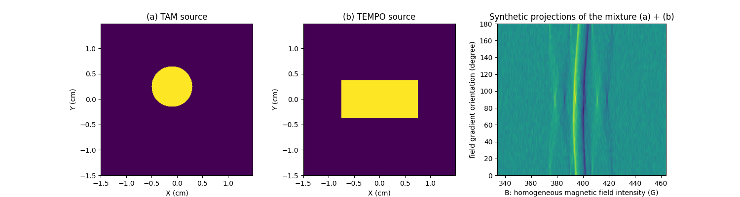
Let us create two synthetic 2D images containing binary shapes (one disk for the first image, and one rectangle for the second one). We will then load two (real) EPR spectra (one spectrum of TAM and one spectrum of TEMPO).

In this synthetic experiment, the first synthetic image (containing the disk) shall represent the 2D concentration mapping of TAM and the second one (containing the rectangle) shall represent the 2D concentration mapping of a TEMPO.

For each species, a synthetic sequence of projection is generated, then the two sequences are summed to simulate the sequence of projections corresponding to a mixture of TAM and TEMPO.

#--------------------------#
# Compute synthetic images #
#--------------------------#

# set datatype, pixel-size & dimensions of the source images
dtype = 'float32'
delta = 1e-2 # spatial sampling step (cm)
Nx, Ny = 300, 300 # width & height of the source images

# compute spatial coordinates
x = (-(Nx//2) + backend.arange(Nx)) * delta
y = (-(Ny//2) + backend.arange(Ny)) * delta
X, Y = backend.meshgrid(x, y)

# compute TAM source image (disk)
D = .8 # disc diameter (cm)
x0, y0 = -0.1, .25 # center coordinates
u_tam = backend.cast((X - x0)**2 + (Y - y0)**2 <= (D/2)**2, dtype)

# compute TEMPO source image (filled rectangle)
rx, ry = 1.5, .75 # rectangle size along each axis (cm)
u_tempo = backend.cast((backend.abs(X) <= rx/2.) &
                       (backend.abs(Y) <= ry/2.), dtype)

#--------------------------------------------------------#
# load TAM & TEMPO reference spectra (real measurements) #
#--------------------------------------------------------#

# retrieve paths towards of the different files comprised in the dataset
path_htam = datasets.get_path('tam-and-tempo-tubes-2d-20210609-htam.pkl') # or use your own dataset, e.g., path_htam = '~/my_tam_spectrum.DSC'
path_htempo = datasets.get_path('tam-and-tempo-tubes-2d-20210609-htempo.pkl') # or use your own dataset, e.g., path_htempo = '~/my_tempo_spectrum.DSC'

# load the dataset in float32 precision
dtype = 'float32'
dataset_htam = io.load(path_htam, backend=backend, dtype=dtype) # load the dataset containing the TAM reference spectrum
dataset_htempo = io.load(path_htempo, backend=backend, dtype=dtype) # load the dataset containing the TEMPO reference spectrum

# extract data from the loaded datasets
B = dataset_htam['B'] # B sampling nodes
h_tam = dataset_htam['DAT'] # reference spectrum of the TAM
h_tempo = dataset_htempo['DAT'] # reference spectrum of the TEMPO

#--------------------------------#
# generate synthetic projections #
#--------------------------------#

# generate field gradient vector
Gampl = 10 # gradient amplitude (G/cm)
Nproj = 40 # number of projections to simulate
theta = backend.linspace(0, math.pi, Nproj, dtype=dtype) # Gradient orientations (rad)
Gx = Gampl * backend.cos(theta)
Gy = Gampl * backend.sin(theta)
fg = backend.stack([Gx, Gy])

# compute synthetic projections as the sum between the projections of
# the TAM source and the projections of the TEMPO source
proj_tam = monosrc.proj2d(u_tam, delta, B, h_tam, fg, backend=backend)
proj_tempo = monosrc.proj2d(u_tempo, delta, B, h_tempo, fg, backend=backend)
proj_mixture = proj_tam + proj_tempo

# add synthetic noise (Gaussian)
proj_mixture += backend.randn(proj_mixture.shape, std=5e3)

#-------------------------------------------------#
# display source images and synthetic projections #
#-------------------------------------------------#

# prepare display
plt.figure(figsize=(15, 4))
img_extent = [t.item() for t in (x[0], x[-1], y[0], y[-1])]
proj_extent = [t.item() for t in (B[0], B[-1], theta[0]*180./math.pi, theta[-1]*180./math.pi)]

# display TAM source image
plt.subplot(1, 3, 1)
plt.imshow(backend.to_numpy(u_tam), extent=img_extent, origin='lower')
plt.title("(a) TAM source")
plt.xlabel("X (cm)")
plt.ylabel("Y (cm)")

# display TEMPO source image
plt.subplot(1, 3, 2)
plt.imshow(backend.to_numpy(u_tempo), extent=img_extent, origin='lower')
plt.title("(b) TEMPO source")
plt.xlabel("X (cm)")
plt.ylabel("Y (cm)")

# synthetic projections of the mixture of TAM + TEMPO
plt.subplot(1, 3, 3)
plt.imshow(backend.to_numpy(proj_mixture), extent=proj_extent, aspect='auto')
plt.title("Synthetic projections of the mixture (a) + (b)")
plt.xlabel("B: homogeneous magnetic field intensity (G)")
_ = plt.ylabel("field gradient orientation (degree)")

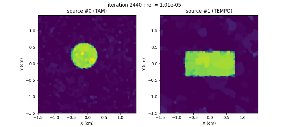
Source separation (reconstruction of the TAM & TEMPO source images)

Now let us perform the source separation, that is, the reconstruction of two 2D images: the concentration mappings of the (simulated) TAM species that of the (simulated) TEMPO species.

# ----------------------------- #
# Set reconstruction parameters #
# ----------------------------- #
tam_shape = (100, 100) # required shape (number of pixels along each axe) for the output TAM source
tempo_shape = (100, 100) # required shape (number of pixels along each axe) for the output TEMPO source
out_shape = (tam_shape, tempo_shape) # output image shape
delta = 3e-2 # sampling step in the same length unit as the provided field gradient coordinates (here cm)
lbda = 10 # normalized regularity parameter (arbitrary unit)
proj = (proj_mixture,) # list of input experiments (here only one experiment)
h = ((h_tam, h_tempo),) # list of source spectra associated to each experiment
fgrad = (fg,) # list of field gradient vectors associated to each experiment

# ----------------------- #
# Set optional parameters #
# ----------------------- #
nitermax = 5000 # maximal number of iterations
verbose = False # disable console verbose mode
video = True # enable video display
Ndisplay = 20 # refresh display rate (iteration per refresh)
eval_energy = False # disable TV-regularized least-square energy
                    # evaluation each Ndisplay iteration

# ---------------------------------------------------------- #
# Customize 2D multi-sources image displayer (optional, used #
# only when video=True above)                                #
# ---------------------------------------------------------- #
tam_shape = out_shape[0]
tempo_shape = out_shape[1]
xgrid_tam = (-(tam_shape[1]//2) + np.arange(tam_shape[1])) * delta
ygrid_tam = (-(tam_shape[0]//2) + np.arange(tam_shape[0])) * delta
xgrid_tempo = (-(tempo_shape[1]//2) + np.arange(tempo_shape[1])) * delta
ygrid_tempo = (-(tempo_shape[0]//2) + np.arange(tempo_shape[0])) * delta
grid_tam = (ygrid_tam, xgrid_tam)
grid_tempo = (ygrid_tempo, xgrid_tempo)
grids = (grid_tam, grid_tempo) # provide spatial sampling grids for each source
unit = 'cm' # provide length unit associated to the grids
display_labels = True # display axes labels within subplots
adjust_dynamic = True # maximize displayed dynamic at each refresh
boundaries = 'same' # give all subplots the same axes boundaries (ensure same pixel size for
                    # each displayed slice)
displayFcn = lambda u : [np.maximum(im, 0) for im in u] # display
                                                        # positive
                                                        # part of each
                                                        # source image
figsize = (10., 4.4) # size of the figure to be displayed
src_labels = ('TAM', 'TEMPO') # source labels (to be included into suptitles)
displayer = displayers.create_2d_displayer(nsrc=2, units=unit,
                                           figsize=figsize,
                                           adjust_dynamic=adjust_dynamic,
                                           display_labels=display_labels,
                                           boundaries=boundaries,
                                           grids=grids,
                                           src_labels=src_labels,
                                           displayFcn=displayFcn)

# --------------------------------------------------------------------- #
# Configure and run the TV-regularized multisource image reconstruction #
# --------------------------------------------------------------------- #
out = processing.tv_multisrc(proj, B, fgrad, delta, h, lbda,
                             out_shape, backend=backend, tol=1e-5,
                             nitermax=nitermax,
                             eval_energy=eval_energy, video=video,
                             verbose=verbose, Ndisplay=Ndisplay,
                             displayer=displayer)

Estimated memory usage: 240 MB