Note
Go to the end to download the full example code.
Separation of a TAM insert in a TEMPO solution (real 3D dataset)
Simultaneous image reconstruction and separation of sample made of one small eppendorf filled with a solution of TAM inserted into a larger eppendorf filled with a solution of TEMPO (see here for the sample and the dataset description).
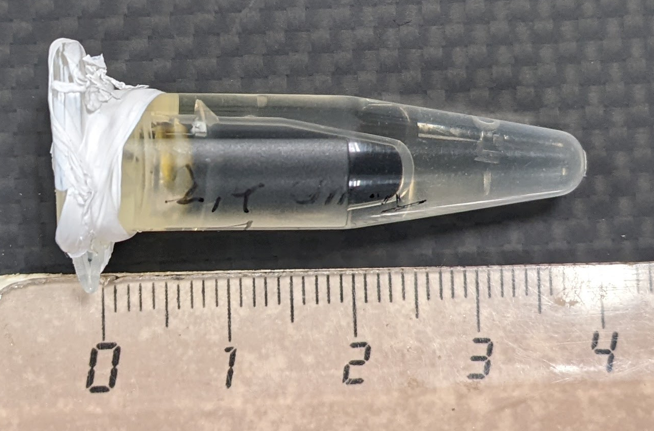
Picture of the sample.
Import needed modules
import math # basic math functions
import numpy as np # for array manipulations
import matplotlib.pyplot as plt # tools for data visualization
import pyepri.backends as backends # to instanciate PyEPRI backends
import pyepri.datasets as datasets # to retrieve the path (on your own machine) of the demo dataset
import pyepri.displayers as displayers # tools for displaying images (with update along the computation)
import pyepri.processing as processing # tools for EPR image reconstruction
import pyepri.io as io # tools for loading EPR datasets (in BES3T or Python .PKL format)
Create backend
We create a numpy backend here because it should be available on your system (as a mandatory dependency of the PyEPRI package). You can try another backend (if available on your system) by uncommenting the appropriate line below (using a GPU backend may drastically reduce the computation time).
backend = backends.create_numpy_backend() # default numpy backend (CPU)
#backend = backends.create_torch_backend('cpu') # uncomment here for torch-cpu backend (CPU)
#backend = backends.create_cupy_backend() # uncomment here for cupy backend (GPU)
#backend = backends.create_torch_backend('cuda') # uncomment here for torch-gpu backend (GPU)
Load the input dataset
We load the tam-insert-in-tempo-20230929 dataset (embedded with
the PyEPRI package) in float32 precision. Take a look to the
comments for changing the precision to float64 or replacing the
embedded dataset by one of your own dataset. Note that to adapt this
example to your own dataset, you will need to provide
the sequence of measured projection of the sample (mixture of multiple EPR species);
the reference spectrum of each EPR species present in the sample (must be calculated beforehand, preferably extracted from the reference spectrum of the mixture).
# set the path towards the measured projections (mixture of TAM & TEMPO)
path_proj = datasets.get_path('tam-insert-in-tempo-20230929-proj.pkl') # or use your own dataset, e.g., path_proj = '~/my_projections.DSC'

# set the paths towards the reference spectra of each EPR species
# present in the mixture (in this dataset, the reference spectra of
# the single species were fited from the ref. spectrum of the mixture)
path_htam = datasets.get_path('tam-insert-in-tempo-20230929-htam.pkl') # or use your own dataset, e.g., path_htam = '~/my_tam_spectrum.DSC'
path_htempo = datasets.get_path('tam-insert-in-tempo-20230929-htempo.pkl') # or use your own dataset, e.g., path_htempo = '~/my_tempo_spectrum.DSC'

# load the dataset in float32 precision
dtype = 'float32' # use 'float32' for single (32 bit) precision and 'float64' for double (64 bit) precision
dataset_proj = io.load(path_proj, backend=backend, dtype=dtype) # load the dataset containing the projections
dataset_htam = io.load(path_htam, backend=backend, dtype=dtype) # load the dataset containing the TAM reference spectrum
dataset_htempo = io.load(path_htempo, backend=backend, dtype=dtype) # load the dataset containing the TEMPO reference spectrum

# extract data from the loaded datasets
B = dataset_proj['B'] # B sampling nodes
proj_mixture = dataset_proj['DAT'] # projections data
fg = dataset_proj['FGRAD'] # field gradient vectors coordinates
h_tam = dataset_htam['DAT'] # reference spectrum of the TAM
h_tempo = dataset_htempo['DAT'] # reference spectrum of the TEMPO
Display the input dataset
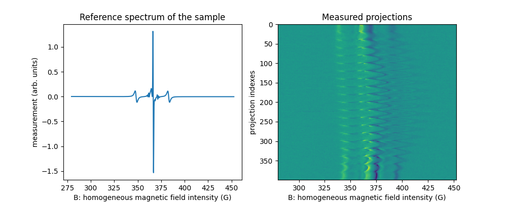
Before addressing the source separation problem, let us take a look at the measured reference spectrum of the sample (TAM + TEMPO mixture) as well as to the measured projections.
# prepare display
plt.figure(figsize=(10, 4))
theta = backend.arctan2(fg[1], fg[0])
proj_extent = [B[0].item(), B[-1].item(), proj_mixture.shape[0] - 1, 0]

# display reference spectrum of the sample (contains one tube of TAM
# and one tube of TEMPO)
plt.subplot(1, 2, 1)
plt.plot(backend.to_numpy(B), backend.to_numpy(h_tam + h_tempo))
plt.xlabel("B: homogeneous magnetic field intensity (G)")
plt.ylabel("measurement (arb. units)")
plt.title("Reference spectrum of the sample")

# display measured projections
plt.subplot(1, 2, 2)
plt.imshow(backend.to_numpy(proj_mixture), extent=proj_extent, aspect='auto')
plt.title("Measured projections")
plt.xlabel("B: homogeneous magnetic field intensity (G)")
plt.ylabel("projection indexes")
plt.show() # to keep the display persistent when the code is executed as a script
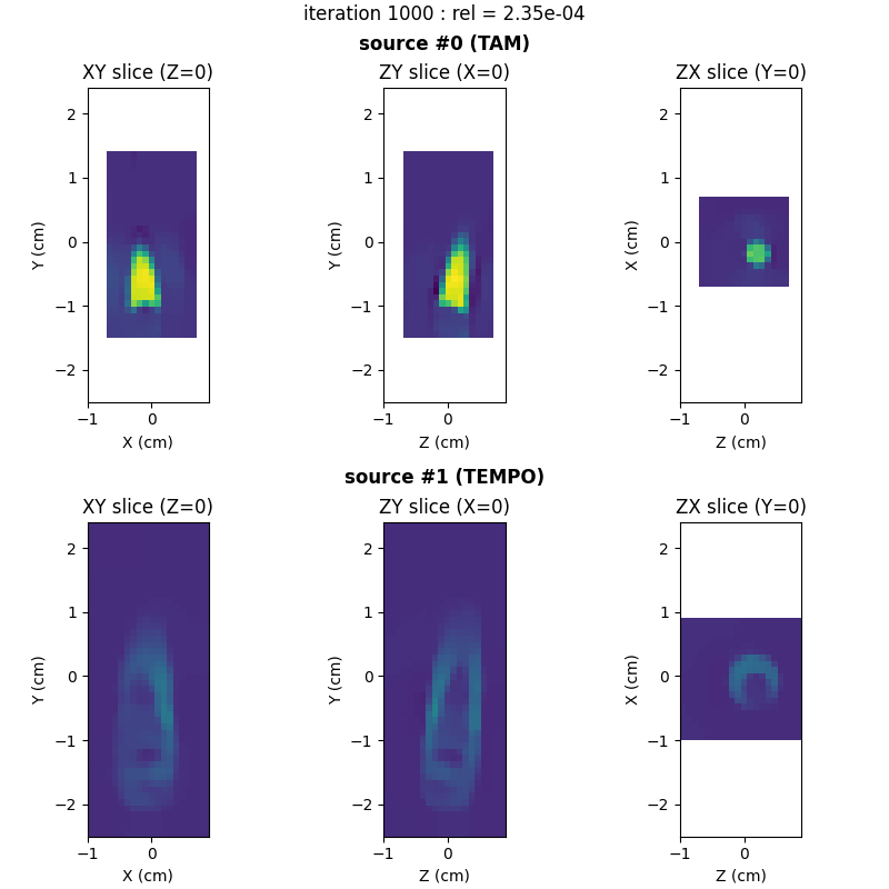
Perform source separation
Now let us perform the source separation, that is, the reconstruction of one image of the tube of TAM and one image of the tube of TEMPO.
# ----------------------------- #
# Set reconstruction parameters #
# ----------------------------- #
tam_shape = (30, 15, 15) # required shape (number of pixels along each axe) for the output TAM source
tempo_shape = (50, 20, 20) # required shape (number of pixels along each axe) for the output TEMPO source
delta = .1 # sampling step in the same length unit as the provided field gradient coordinates (here cm)
lbda = 2e-5 # regularity parameter (arbitrary unit)
out_shape = (tam_shape, tempo_shape) # output image shape
proj = (proj_mixture,) # list of input experiments (here only one experiment)
h = ((h_tam, h_tempo),) # list of source spectra associated to each experiment
fgrad = (fg,) # list of field gradient vectors associated to each experiment

# ----------------------- #
# Set optional parameters #
# ----------------------- #
nitermax = 1000 # maximal number of iterations
verbose = False # disable console verbose mode
video = True # enable video display
Ndisplay = 10 # refresh display rate (iteration per refresh)
eval_energy = False # disable TV-regularized least-square energy
                    # evaluation each Ndisplay iteration

# ---------------------------------------------------------- #
# Customize 3D multi-sources image displayer (optional, used #
# only when video=True above)                                #
# ---------------------------------------------------------- #
tam_shape = out_shape[0]
tempo_shape = out_shape[1]
xgrid_tam = (-(tam_shape[1]//2) + np.arange(tam_shape[1])) * delta
ygrid_tam = (-(tam_shape[0]//2) + np.arange(tam_shape[0])) * delta
zgrid_tam = (-(tam_shape[2]//2) + np.arange(tam_shape[2])) * delta
xgrid_tempo = (-(tempo_shape[1]//2) + np.arange(tempo_shape[1])) * delta
ygrid_tempo = (-(tempo_shape[0]//2) + np.arange(tempo_shape[0])) * delta
zgrid_tempo = (-(tempo_shape[2]//2) + np.arange(tempo_shape[2])) * delta
grid_tam = (ygrid_tam, xgrid_tam, zgrid_tam)
grid_tempo = (ygrid_tempo, xgrid_tempo, zgrid_tempo)
grids = (grid_tam, grid_tempo) # provide spatial sampling grids for each source
unit = 'cm' # provide length unit associated to the grids
display_labels = True # display axes labels within subplots
adjust_dynamic = True # maximize displayed dynamic at each refresh
origin = "lower"
boundaries = 'same' # give all subplots the same axes boundaries (ensure same pixel size for
                    # each displayed slice)
src_labels = ('TAM', 'TEMPO') # source labels (to be included into suptitles)
figsize = (8., 8.) # size of the figure to be displayed
displayer = displayers.create_3d_displayer(nsrc=2,
                                           units=unit,
                                           figsize=figsize,
                                           adjust_dynamic=adjust_dynamic,
                                           display_labels=display_labels,
                                           boundaries=boundaries,
                                           origin=origin, grids=grids,
                                           src_labels=src_labels)

# --------------------------------------------------------------------- #
# Configure and run the TV-regularized multisource image reconstruction #
# --------------------------------------------------------------------- #
out = processing.tv_multisrc(proj, B, fgrad, delta, h, lbda,
                             out_shape, backend=backend, tol=1e-5,
                             nitermax=nitermax,
                             eval_energy=eval_energy, video=video,
                             verbose=verbose, Ndisplay=Ndisplay,
                             displayer=displayer)
plt.show() # to keep the display persistent when the code is executed as a script
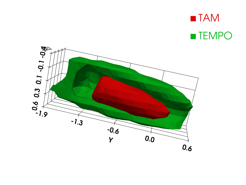
Isosurface rendering (requires working pyvista installation)
Let us display isosurfaces of the reconstructed TAM and TEMPO source images (TAM is displayed in red color and TEMPO is displayed in green color). The TEMPO source image is masked over half a plane so that we can visualize the TAM insert.
# additional import (pyvista)
import pyvista as pv # tools for rendering 3D volumes

# prepare isosurface display
x_tam, y_tam, z_tam = np.meshgrid(xgrid_tam, ygrid_tam, zgrid_tam, indexing='xy')
x_tempo, y_tempo, z_tempo = np.meshgrid(xgrid_tempo, ygrid_tempo, zgrid_tempo, indexing='xy')
grid_tam = pv.StructuredGrid(x_tam, y_tam, z_tam)
grid_tempo = pv.StructuredGrid(x_tempo, y_tempo, z_tempo)

# compute TAM isosurface
vol = np.moveaxis(backend.to_numpy(out[0]), (0,1,2), (2,1,0))
grid_tam["vol"] = vol.flatten()
l1 = vol.max()
l0 = .5 * l1
isolevels = np.linspace(l0, l1, 10)
contours_tam = grid_tam.contour(isolevels)

# compute TEMPO isosurface (mask half of the reconstructed volume so
# that we can see inside)
mask = (x_tempo > -.3).astype(dtype)
vol_left = backend.to_numpy(out[1]) * mask
vol_left = np.moveaxis(vol_left, (0,1,2), (2,1,0))
grid_tempo["vol"] = vol_left.flatten()
l0 = 0.11 * l1
isolevels = np.linspace(l0, l1, 10)
contours_tempo = grid_tempo.contour(isolevels)

# display isosurfaces (green = TAM, red = TEMPO)
p = pv.Plotter()
cpos = [(-5.92, -0.11, -1.35), (-0.02, -0.62, 0.1), (0.22, -0.22, -0.95)]
p.camera_position = cpos
labels = dict(ztitle='Z', xtitle='X', ytitle='Y')
p.add_mesh(contours_tam, show_scalar_bar=False, color='#db0404', label=' TAM')
p.add_mesh(contours_tempo, show_scalar_bar=False, color='#01b517', label=' TEMPO')
p.show_grid(**labels)
p.add_legend(face='r')
p.show()
Total running time of the script: (0 minutes 22.225 seconds)
Estimated memory usage: 262 MB