Projection operators

Presentation of the projection operators (core low-level components of this package).

EPR acquisitions can be linked to the spatial mapping (or image) of the concentration of the paramagnetic species present in the cavity of the acquisition system through a specific projection operation. The accurate modeling of the projection operators as well as their efficient implementations is of crucial importance to address accurate and efficient processing of the EPR acquisition. This is particularly the case when addressing the inverse problem of EPR image reconstruction with variational models.

This package currently implements projection operators suited to various situations (single or multiple EPR sources, 2D or 3D setting). Usage example and recommendations are described below.

Single EPR source (2D setting)

The functions pyepri.monosrc.proj2d() takes as input the 2D image of a single EPR species, its reference spectrum, and a sequence of 2D field gradient vector coordinates (in the image plane), it returns a sequence of 2D projections (2D sinogram).

A synthetic projection experiment in this framework is provided below.

# -------------- #
# Import modules #
# -------------- #
import math
import matplotlib.pyplot as plt
import numpy as np
import pyepri.backends as backends
import pyepri.monosrc as monosrc
import pyepri.multisrc as multisrc
import pyvista as pv
plt.ion()

# -------------- #
# Create backend #
# -------------- #
#
# You can uncomment one line below to select another backend (if
# installed on your system).
#
backend = backends.create_numpy_backend()
#backend = backends.create_torch_backend('cpu') # uncomment here for torch-cpu backend
#backend = backends.create_cupy_backend() # uncomment here for cupy backend
#backend = backends.create_torch_backend('cuda') # uncomment here for torch-gpu backend

# -------------------------------------------------------------- #
# Compute synthetic inputs (2D image, reference spectrum & field #
# gradient vector coordinates)                                   #
# -------------------------------------------------------------- #

# synthetic 2D image
dtype = 'float32'
delta = 5e-3 # sampling step (cm)
Nx, Ny = 550, 400 # image size
xgrid = (-(Nx//2) + backend.arange(Nx, dtype=dtype)) * delta # sampling grid along the X-axis
ygrid = (-(Ny//2) + backend.arange(Ny, dtype=dtype)) * delta # sampling grid along the Y-axis
X, Y = backend.meshgrid(xgrid, ygrid) # spatial sampling grid
u1 = backend.cast(((X - .2)**2 + (Y + .2)**2 <= .08**2), dtype)
u2 = backend.cast((X + .2)**2 + (Y - .2)**2 <= .08**2, dtype)
u3 = backend.cast((X + .2)**2 + (Y + .2)**2 <= .05**2, dtype)
u4 = backend.cast((X - .2)**2 + (Y - .2)**2 <= .05**2, dtype)
u = u1 + u2 + u3 + u4
u /= (delta ** 2) * u.sum()

# synthetic reference spectrum (simple Gaussian derivative)
B = backend.linspace(380, 420, 512, dtype=dtype)
Br = 400
sig = .3
cof = 1. / (sig * math.sqrt(2. * math.pi))
h = - cof * (B - Br) / sig**2 * backend.exp(- (B - Br)**2 / (2. * sig**2))

# field gradient vector coordinates (one vector per projection to
# compute)
theta = backend.linspace(0, 2. * math.pi, 100, dtype=dtype) # field gradient orientations
mu = 20 # field gradient amplitude (G/cm)
gx = mu * backend.cos(theta) # X-axis coordinates of the field gradient vectors
gy = mu * backend.sin(theta) # Y-axis coordinates of the field gradient vectors
fgrad = backend.stack((gx, gy))

# ----------------------------- #
# Compute synthetic projections #
# ----------------------------- #
proj = monosrc.proj2d(u, delta, B, h, fgrad, backend=backend)

# ---------------------------- #
# Display signals (u, h, proj) #
# ---------------------------- #

# input image
plt.figure(figsize=(19.5, 4.2))
plt.subplot(1, 3, 1)
extent = [t.item() for t in (xgrid[0], xgrid[-1], ygrid[0], ygrid[-1])]
plt.imshow(backend.to_numpy(u), extent=extent, origin='lower')
plt.xlabel('X (cm)')
plt.ylabel('Y (cm)')
plt.title('input image')

# input reference spectrum
plt.subplot(1, 3, 2)
plt.plot(backend.to_numpy(B), backend.to_numpy(h))
plt.grid(linestyle=':')
plt.xlabel('B: homogeneous magnetic field (G)')
plt.ylabel('spectrum (arb. unit)')
plt.title('input reference spectrum')

# computed projections
plt.subplot(1, 3, 3)
extent = (B[0].item(), B[-1].item(), proj.shape[0] - 1, 0)
plt.imshow(backend.to_numpy(proj), extent=extent, aspect='auto')
plt.xlabel('B: homogeneous magnetic field (G)')
plt.ylabel('projection index')
_ = plt.title('output sequence of projections (sinogram)')

Remark: in the above synthetic experiment, all generated projections were computed using a magnetic field gradient with fixed amplitude (mu = 20 G/cm), only the orientation of the magnetic field gradient vector changes from one projection to another. Computing projections with non constant magnetic field gradient amplitude is also possible as there is no constraint on the coordinates of the magnetic field gradient vectors passed as input parameter (fgrad), as we shall illustrate now.

# ----------------------------------------------------------------- #
# Compute field gradient vector coordinates with non constant field #
# gradient amplitudes                                               #
# ----------------------------------------------------------------- #
theta = backend.linspace(0, 2. * math.pi, 100, dtype=dtype)
mu = backend.from_numpy(np.array([20., 40.], dtype=dtype).reshape((-1, 1)))
gx = (mu * backend.cos(theta)).reshape((-1,))
gy = (mu * backend.sin(theta)).reshape((-1,))
fgrad = backend.stack((gx, gy))

# ----------------------------- #
# compute synthetic projections #
# ----------------------------- #
proj = monosrc.proj2d(u, delta, B, h, fgrad, backend)

# ---------------------------------------------------------- #
# Display field gradient orientations & computed projections #
# ---------------------------------------------------------- #

# magnetic field gradient orientations
plt.figure(figsize=(16., 7.))
plt.subplot(1, 2, 1)
s = plt.scatter(backend.to_numpy(fgrad[0]), backend.to_numpy(fgrad[1]), s=5)
plt.grid(linestyle=':')
s.axes.set_aspect('equal', 'box')
plt.xlabel('X (cm)')
plt.ylabel('Y (cm)')
plt.title('magnetic field gradient samples')

# computed projections
plt.subplot(1, 2, 2)
extent = (B[0].item(), B[-1].item(), proj.shape[0] - 1, 0)
plt.imshow(backend.to_numpy(proj), extent=extent, aspect='auto')
plt.xlabel('B: homogeneous magnetic field (G)')
plt.ylabel('projection index')
_ = plt.title('output sequence of projections (sinogram)')

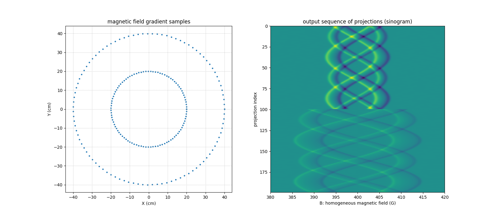
WARNING: when computing the projections, the user must make sure that the acquisition range for the homogeneous magnetic field intensity values B provided as input is large enough to support all the computed projections. This means that the real projections should vanish outside from this range. Otherwise, non-realistic projections are computed due to aliasing artifacts that occur in the B-domain (see below, where we reproduce the first experiment using a restricted range for the input B).

# ------------------------------------------------------------------ #
# Regenerate the first experiment (use a large enough B range first) #
# ------------------------------------------------------------------ #

# synthetic reference spectrum (simple Gaussian derivative)
B = backend.linspace(380, 420, 512, dtype=dtype)
Br = 400
sig = .3
cof = 1. / (sig * math.sqrt(2. * math.pi))
h = - cof * (B - Br) / sig**2 * backend.exp(- (B - Br)**2 / (2. * sig**2))

# field gradient vector coordinates (one vector per projection to
# compute)
theta = backend.linspace(0, 2. * math.pi, 100, dtype=dtype) # field gradient orientations
mu = 20. # field gradient amplitude (G/cm)
gx = mu * backend.cos(theta) # X-axis coordinates of the field gradient vectors
gy = mu * backend.sin(theta) # Y-axis coordinates of the field gradient vectors
fgrad = backend.stack((gx, gy))

# compute synthetic projections
proj1 = monosrc.proj2d(u, delta, B, h, fgrad, backend=backend)

# ------------------------------------------------------------------- #
# Now restrict the range of the input B and recompute the projections #
# (aliasing will occur, leading to non realistic projections)         #
# ------------------------------------------------------------------- #

# restrict input B domain
B2 = B[190:310]
h2 = h[190:310]

# recompute synthetic projections (aliasing occurs here)
proj2 = monosrc.proj2d(u, delta, B2, h2, fgrad, backend=backend)

# -------------------------------------------- #
# Display and compare the computed projections #
# -------------------------------------------- #

# projections computed with large-enough B range
plt.figure(figsize=(11.15, 4.))
plt.subplot(1, 2, 1)
extent = (B[0].item(), B[-1].item(), proj1.shape[0] - 1, 0)
hdl1 = plt.imshow(backend.to_numpy(proj1), extent=extent, aspect='auto')
plt.xlabel('B: homogeneous magnetic field (G)')
plt.ylabel('projection index')
_ = plt.title('Realistic projections (B-range is large enough)')

# projections computed with too small B range
plt.subplot(1, 2, 2)
extent = (B2[0].item(), B2[-1].item(), proj2.shape[0] - 1, 0)
hdl2 = plt.imshow(backend.to_numpy(proj2), extent=extent, aspect='auto')
hdl2.axes.set_xlim(hdl1.axes.get_xlim())
plt.xlabel('B: homogeneous magnetic field (G)')
plt.ylabel('projection index')
_ = plt.title('Non-realistic projections (B-range is too small)')

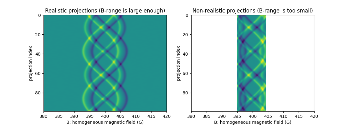
With real-life measurements, one would expect the projections measured over the restricted B-range to correspond to a cropping of the projections measured over the larger B-range. This is not what we observe above since the signal of the left-hand side image outside from the restricted area is still present in the right-hand side image in an aliasing fashion (the signal that should be cropped outside from one side of the image re-enters through the other side). Consequently, when a too small B-range is used, the pyepri.monosrc.proj2d() operator does not faithfully describe the relation between the latent image and the real-life projections. Relying on such operator (with a too small B-range) to process real-life measurements (for instance to perform image reconstruction) would fatally lead to artifacts in the reconstructed signal.

Single EPR source (3D setting)

The function pyepri.monosrc.proj3d() takes as input the 3D image of a single EPR species, its reference spectrum, and a sequence of 3D field gradient vector coordinates, it returns a sequence of 3D projections (3D sinogram).

Now, let us perform a synthetic projection experiment under this framework is provided below. First, let us compute and display a synthetic 3D image made of two ellipsoids (those shape may represent for instance two tubes filled with a paramagnetic solution).

# --------------------------------------------------------- #
# Compute a synthetic 3D input image made of two ellipsoids #
# --------------------------------------------------------- #
Nx, Ny, Nz = 128, 256, 128 # image dimensions
delta = .02 # spatial sampling step (cm)
xgrid = (-(Nx//2) + backend.arange(Nx, dtype=dtype)) * delta
ygrid = (-(Ny//2) + backend.arange(Ny, dtype=dtype)) * delta
zgrid = (-(Nz//2) + backend.arange(Nz, dtype=dtype)) * delta
X, Y, Z = backend.meshgrid(xgrid, ygrid, zgrid)
v1 = (((X - .4) / .25)**2 + ((Y - .1) / .7)**2 + (((Z - .4) / .25)**2) <= 1.)
v2 = (((X + .4) / .25)**2 + ((Y + .1) / .9)**2 + (((Z + .4) / .25)**2) <= 1.)
v = backend.cast(v1, dtype) + backend.cast(v2, dtype)
v /= (delta**3 * v.sum())

# ----------------------------------- #
# Display input 3D image (isosurface) #
# ----------------------------------- #

# compute isosurface sampling grid
grid = pv.StructuredGrid(backend.to_numpy(X), backend.to_numpy(Y), backend.to_numpy(Z))

# compute isosurface
vol = np.moveaxis(backend.to_numpy(v), (0,1,2), (2,1,0))
grid["vol"] = vol.flatten()
l1 = vol.max()
l0 = .2 * l1
isolevels = np.linspace(l0, l1, 10)
contours = grid.contour(isolevels)

# display isosurface
cpos = [(-3.8, 4.35, 2.11), (0.0, -0.1, 0.0), (-0.33, -0.62, 0.71)]
p = pv.Plotter()
p.camera_position = cpos
labels = dict(ztitle='Z', xtitle='X', ytitle='Y')
p.add_mesh(contours, show_scalar_bar=False, color='#f7fe00')
p.show_grid(**labels)
p.show()

Static Scene

Interactive Scene

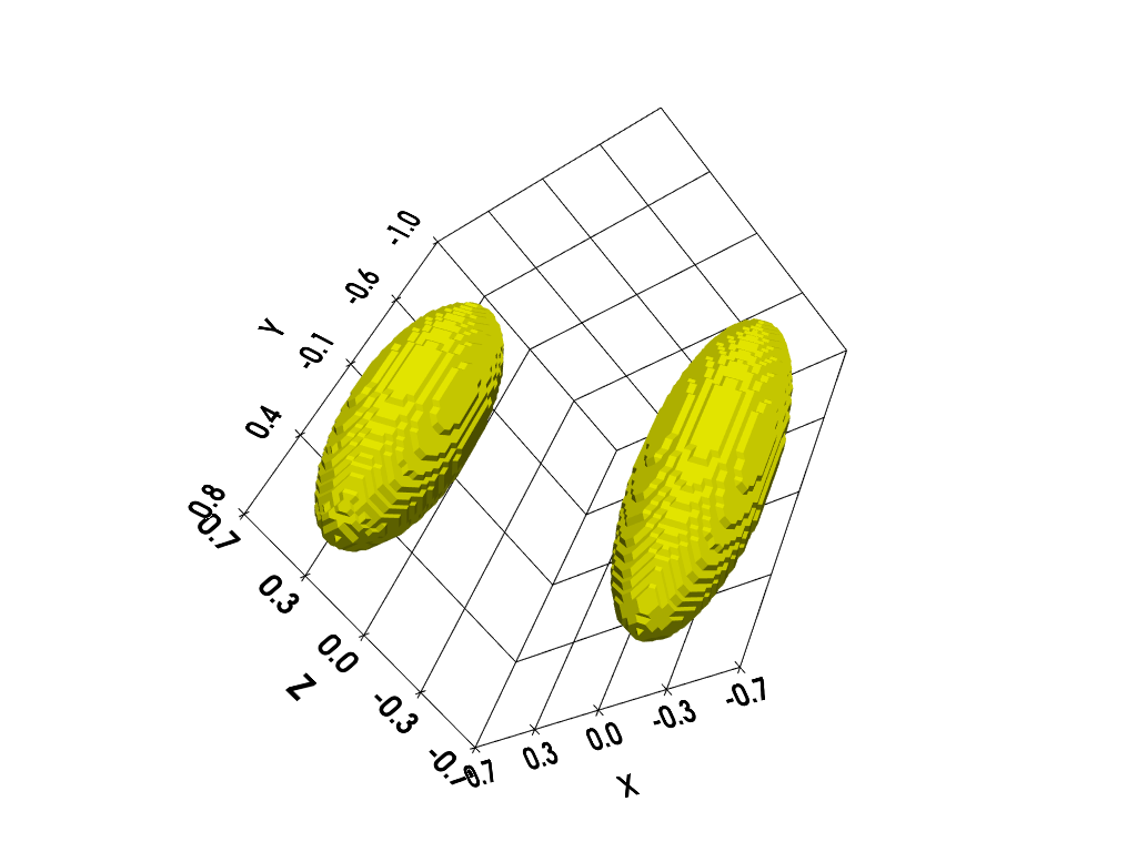
Next, let us synthesize the remaining inputs (reference spectrum and field gradient vector coordinates).

# ------------------------------------------------------------ #
# Compute synthetic reference spectrum & field gradient vector #
# coordinates                                                  #
# ------------------------------------------------------------ #

# synthetic reference spectrum (simple Gaussian derivative)
B = backend.linspace(370, 430, 512, dtype=dtype)
Br = 400
sig = .3
cof = 1. / (sig * math.sqrt(2. * math.pi))
h = - cof * (B - Br) / sig**2 * backend.exp(- (B - Br)**2 / (2. * sig**2))

# field gradient vector coordinates
t1 = backend.linspace(0, 2. * math.pi, 32, dtype=dtype)
t2 = backend.linspace(0, 2. * math.pi, 32, dtype=dtype)
theta1, theta2 = backend.meshgrid(t1, t2)
theta1 = theta1.reshape((-1,)) # polar angles of the field gradients
theta2 = theta2.reshape((-1,)) # azimuthal angles of the field gradients
mu = 20 # field gradient amplitude (G/cm)
gx = mu * backend.cos(theta1) * backend.sin(theta2) # X-axis coordinates of the field gradient vectors
gy = mu * backend.sin(theta1) * backend.sin(theta2) # Y-axis coordinates of the field gradient vectors
gz = mu * backend.cos(theta2) # Z-axis coordinates of the field gradient vectors
fgrad = backend.stack((gx, gy, gz))

# ------- #
# Display #
# ------- #

# reference spectrum
fig = plt.figure(figsize=(8.8, 4.))
fig.add_subplot(1, 2, 1)
plt.plot(backend.to_numpy(B), backend.to_numpy(h))
plt.grid(linestyle=':')
plt.xlabel('B: homogeneous magnetic field (G)')
plt.ylabel('spectrum (arb. unit)')
plt.title('input reference spectrum')

# magnetic field gradient vectors
ax = fig.add_subplot(1, 2, 2, projection='3d')
ax.scatter(backend.to_numpy(fgrad[0]), backend.to_numpy(fgrad[1]), backend.to_numpy(fgrad[2]))
ax.set_xlabel('X (cm)')
ax.set_ylabel('Y (cm)')
ax.set_zlabel('Z (cm)')
ax.set_aspect('equal', 'box')
_ = plt.title('magnetic field gradient samples')

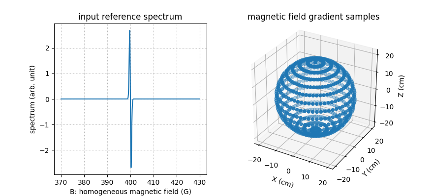
Finally, we can compute and display the projections of the 3D image.

# ------------------- #
# Compute projections #
# ------------------- #
proj = monosrc.proj3d(v, delta, B, h, fgrad, backend=backend)

# ------------------- #
# Display projections #
# ------------------- #
plt.figure(figsize=(9.6, 5.2))
extent = (B[0].item(), B[-1].item(), proj.shape[0] - 1, 0)
plt.imshow(backend.to_numpy(proj), extent=extent, aspect='auto')
plt.xlabel('B: homogeneous magnetic field (G)')
plt.ylabel('projection index')
_ = plt.title('output sequence of projections (sinogram)')

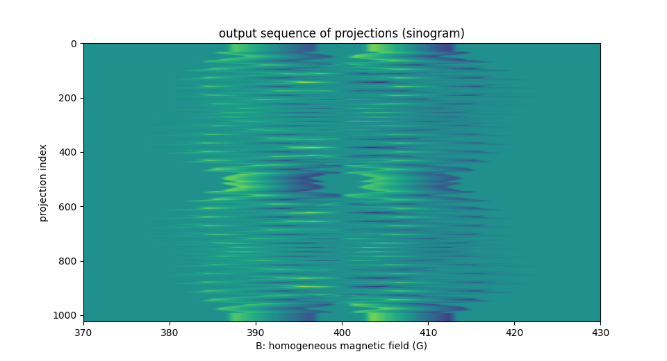
Again, generating projections with variable field gradient amplitudes is easy to do, one simply needs to provide the corresponding field gradient vector coordinates as input of the projection operator. Besides, as in the 2D setting, the user must ensure that the acquisition range for the homogeneous magnetic field intensity values B provided as input is large enough to support all the computed projections.

Multiple EPR sources (2D setting)

When the resonator cavity of the acquisition system contains more than one single type of paramagnetic species, the measured projections can be decomposed as the sum of the contribution of each individual paramagnetic species contained in the sample of interest. This package provides efficient implementations of the projection operator in such situation.

The function pyepri.multisrc.proj2d() takes as input a sequence of 2D images of the individual paramagnetic species (one image per paramagnetic species present in the sample), the sequence of reference spectra of each individual paramagnetic species (one spectrum per paramagnetic species) and a sequence of 2D field gradient vector coordinates (in the image plane), it returns a sequence of 2D projections (2D sinogram) of the sample (mixture of paramagnetic species).

We provide below a synthetic example in the two-dimensional setting of projections computed from a synthetic sample containing two different (synthetic) paramagnetic species.

# ------------------------------------------------------------------ #
# Compute synthetic image of the first EPR source (one disk) and its #
# associated reference spectrum (one single line)                    #
# ------------------------------------------------------------------ #

# synthetic 2D image of the first EPR source (disk)
dtype = 'float32'
delta = 5e-3 # sampling step (cm)
Nx, Ny = 550, 400 # image size
xgrid = (-(Nx//2) + backend.arange(Nx, dtype=dtype)) * delta # sampling grid along the X-axis
ygrid = (-(Ny//2) + backend.arange(Ny, dtype=dtype)) * delta # sampling grid along the Y-axis
X, Y = backend.meshgrid(xgrid, ygrid) # spatial sampling grid
u1 = backend.cast(((X + .3)**2 + (Y - .2)**2 <= .1**2), dtype)
u1 /= (delta ** 2) * u1.sum()

# synthetic reference spectrum of the first EPR source (one line
# spectrum synthesized as the derivative of a Gaussian function)
B = backend.linspace(360, 440, 1200, dtype=dtype)
Br1 = 399
sig1 = .36
cof1 = 1. / (sig1 * math.sqrt(2. * math.pi))
h1 = - cof1 * (B - Br1) / sig1**2 * backend.exp(- (B - Br1)**2 / (2. * sig1**2))

# --------------------------------------------------------------- #
# Compute synthetic image of the second EPR source (another disk) #
# and its associated reference spectrum (three lines spectrum)    #
# --------------------------------------------------------------- #

# synthetic 2D image of the second EPR source (disk)
u2 = backend.cast(((X - .3)**2 + (Y + .2)**2 <= .1**2), dtype)
u2 /= (delta ** 2) * u2.sum()

# synthetic reference spectrum of the second EPR source (three line
# spectrum computed by summing shifted Gaussian derivatives)
Br2_left = 382
Br2_middle = 398
Br2_right = 414
sig2 = .8
cof2 = 1. / (3. * sig2 * math.sqrt(2. * math.pi))
h2_left = - cof2 * (B - Br2_left) / sig2**2 * backend.exp(- (B - Br2_left)**2 / (2. * sig2**2))
h2_middle = - cof2 * (B - Br2_middle) / sig2**2 * backend.exp(- (B - Br2_middle)**2 / (2. * sig2**2))
h2_right = - cof2 * (B - Br2_right) / sig2**2 * backend.exp(- (B - Br2_right)**2 / (2. * sig2**2))
h2 = h2_left + h2_middle + h2_right

# -------------------------------------------------------------------- #
# Compute field gradient vector coordinates (one vector per projection #
# to compute)                                                          #
# -------------------------------------------------------------------- #
theta = backend.linspace(0, 2. * math.pi, 100, dtype=dtype) # field gradient orientations
mu = 20 # field gradient amplitude (G/cm)
gx = mu * backend.cos(theta) # X-axis coordinates of the field gradient vectors
gy = mu * backend.sin(theta) # Y-axis coordinates of the field gradient vectors
fgrad = backend.stack((gx, gy))

# --------------------------------------------------- #
# Compute projections of the multisources EPR mixture #
# --------------------------------------------------- #
proj = multisrc.proj2d((u1, u2), delta, B, ((h1, h2),), (fgrad,), backend=backend)[0]

# -------------------------------------------------------------- #
# Display input images, reference spectra & computed projections #
# -------------------------------------------------------------- #

# prepare display
fig = plt.figure(layout='constrained', figsize=(14., 4.))
subfigs = fig.subfigures(1, 2, wspace=0.07)
ax_left = subfigs[0].subplots(2, 2)
ax_right = subfigs[1].subplots(1, 1)
#clim = [min(u1.min().item(), u2.min().item()), max(u1.max().item(), u2.max().item())]

# first EPR source image
extent = [t.item() for t in (xgrid[0], xgrid[-1], ygrid[0], ygrid[-1])]
im1 = ax_left[0][0].imshow(backend.to_numpy(u1), extent=extent, origin='lower')
ax_left[0][0].set_xlabel('X (cm)')
ax_left[0][0].set_ylabel('Y (cm)')
ax_left[0][0].set_title('image source #1')
#im1.set_clim(clim)
#subfigs[0].colorbar(im1)

# first EPR source reference spectrum
ax_left[0][1].plot(backend.to_numpy(B), backend.to_numpy(h1))
ax_left[0][1].set_xlabel('B: homogeneous magnetic field (G)')
ax_left[0][1].set_ylabel('spectrum (arb. unit)')
ax_left[0][1].set_title('reference spectrum source #1')

# second EPR source image
extent = [t.item() for t in (xgrid[0], xgrid[-1], ygrid[0], ygrid[-1])]
im2 = ax_left[1][0].imshow(backend.to_numpy(u2), extent=extent, origin='lower')
ax_left[1][0].set_xlabel('X (cm)')
ax_left[1][0].set_ylabel('Y (cm)')
ax_left[1][0].set_title('image source #2')
#im2.set_clim(clim)
#subfigs[0].colorbar(im2)

# second EPR source reference spectrum
ax_left[1][1].plot(backend.to_numpy(B), backend.to_numpy(h2))
ax_left[1][1].set_ylim(ax_left[0][1].get_ylim())
ax_left[1][1].set_xlabel('B: homogeneous magnetic field (G)')
ax_left[1][1].set_ylabel('spectrum (arb. unit)')
ax_left[1][1].set_title('reference spectrum source #2')

# computed projections
extent = (B[0].item(), B[-1].item(), proj.shape[0] - 1, 0)
ax_right.imshow(backend.to_numpy(proj), extent=extent, aspect='auto')
ax_right.set_xlabel('B: homogeneous magnetic field (G)')
ax_right.set_ylabel('projection index')
_ = ax_right.set_title('output sequence of projections (sinogram)')

As we can see in this simple synthetic example, the reference spectrum of the first source is made of a single sharp line and the reference spectrum of the second source is made of three lines with larger linewidth than that of the first source. The above displayed sinogram generated from the mixture of the two synthetic EPR sources is comprised of the two contributions of those two synthetic EPR sources. Thanks to the simple shapes of the sources images (both are made of a simple disk) and their spectra, the generated sinogram is rather simple, it exhibits four ribbons shapes and the contribution of the two sources can be clearly distinguished: the contribution of source #1 corresponds to the bright and sharp ribbon shape while the contribution of source #2 corresponds to the three blurry and parallel ribbon shapes visible in the sinogram.

The interest of having such multi-sources projection operator implemented is that it can be used to address the inverse problem of recovering the distinct images of the individual sources from the measured sinogram of the source mixture (some demonstration examples are available in the source separation gallery).

An important feature of the multi-sources operators provided in the PyEPRI package is the ability to simulate at once projections corresponding to various experimental settings. Let us say for instance that we perform two sinograms acquisitions using two different setting of the microwave power. Changing the microwave power will affect in different ways the reference spectra of the individual EPR sources as well as the measured projections. The function pyepri.multisrc.proj2d() is able to generate projections in this situation. To that aim, the user must provide, for each experimental setting, a sequence containing the reference spectra of the individual sources and a sequence containing the field gradient vector coordinates. In this particular example, there are two different experimental settings (one per value of microwave power), so the user must provide h = (h_exp1, h_exp2) and fgrad = (fgrad_exp1, fgrad_exp2) such that:

• h_exp1 = (h1_exp1, h2_exp1, ... hK_exp1) containing the reference spectra of the K individual EPR species at the first value of microwave power (exp1);

• h_exp2 = (h1_exp2, h2_exp2, ... hK_exp2) containing the reference spectra of the N individual EPR species at the second value of microwave power (exp2);

• fgrad_exp1 corresponds to the field gradient vector coordinates to be used to generate the projection in the first experiment (exp1);

• fgrad_exp2 corresponds to the field gradient vector coordinates to be used to generate the projection in the second experiment (exp2);

A synthetic example is provided below (the effect of changing the microwave power is simply modeled by a dilatation of the reference spectrum of each individual EPR source).

# ------------------------------------------------------------------ #
# Compute synthetic image of the first EPR source (one disk) and its #
# associated reference spectrum (one single line) in two different   #
# experimental settings                                              #
# ------------------------------------------------------------------ #

# synthetic 2D image of the first EPR source (disk)
dtype = 'float32'
delta = 5e-3 # sampling step (cm)
Nx, Ny = 550, 400 # image size
xgrid = (-(Nx//2) + backend.arange(Nx, dtype=dtype)) * delta # sampling grid along the X-axis
ygrid = (-(Ny//2) + backend.arange(Ny, dtype=dtype)) * delta # sampling grid along the Y-axis
X, Y = backend.meshgrid(xgrid, ygrid) # spatial sampling grid
u1 = backend.cast(((X + .3)**2 + (Y - .2)**2 <= .1**2), dtype)
u1 /= (delta ** 2) * u1.sum()

# synthetic reference spectrum of the first EPR source (one line
# spectrum synthesized as the derivative of a Gaussian function) in
# the first experimental setting
B = backend.linspace(360, 440, 1200, dtype=dtype)
Br1 = 399
sig1_exp1 = .36
cof1_exp1 = 1. / (sig1_exp1 * math.sqrt(2. * math.pi))
h1_exp1 = - cof1_exp1 * (B - Br1) / sig1_exp1**2 * backend.exp(- (B - Br1)**2 / (2. * sig1_exp1**2))

# synthetic reference spectrum of the first EPR source in the second
# experimental setting (dilatation)
sig1_exp2 = 1.5 * sig1_exp1
cof1_exp2 = 1. / (sig1_exp2 * math.sqrt(2. * math.pi))
h1_exp2 = - cof1_exp2 * (B - Br1) / sig1_exp2**2 * backend.exp(- (B - Br1)**2 / (2. * sig1_exp2**2))

# --------------------------------------------------------------- #
# Compute synthetic image of the second EPR source (another disk) #
# and its associated reference spectrum (three lines spectrum)    #
# --------------------------------------------------------------- #

# synthetic 2D image of the second EPR source (disk)
u2 = backend.cast(((X - .3)**2 + (Y + .2)**2 <= .1**2), dtype)
u2 /= (delta ** 2) * u2.sum()

# synthetic reference spectrum of the second EPR source (three line
# spectrum computed by summing shifted Gaussian derivatives) in the
# first experimental setting
Br2_left = 382
Br2_middle = 398
Br2_right = 414
sig2_exp1 = .8
cof2_exp1 = 1. / (3. * sig2_exp1 * math.sqrt(2. * math.pi))
h2_left_exp1 = - cof2_exp1 * (B - Br2_left) / sig2_exp1**2 * backend.exp(- (B - Br2_left)**2 / (2. * sig2_exp1**2))
h2_middle_exp1 = - cof2_exp1 * (B - Br2_middle) / sig2_exp1**2 * backend.exp(- (B - Br2_middle)**2 / (2. * sig2_exp1**2))
h2_right_exp1 = - cof2_exp1 * (B - Br2_right) / sig2_exp1**2 * backend.exp(- (B - Br2_right)**2 / (2. * sig2_exp1**2))
h2_exp1 = h2_left_exp1 + h2_middle_exp1 + h2_right_exp1

# synthetic reference spectrum of the second EPR source in the second
# experimental setting
sig2_exp2 = 3. * sig2_exp1
cof2_exp2 = 1. / (3. * sig2_exp2 * math.sqrt(2. * math.pi))
h2_left_exp2 = - cof2_exp2 * (B - Br2_left) / sig2_exp2**2 * backend.exp(- (B - Br2_left)**2 / (2. * sig2_exp2**2))
h2_middle_exp2 = - cof2_exp2 * (B - Br2_middle) / sig2_exp2**2 * backend.exp(- (B - Br2_middle)**2 / (2. * sig2_exp2**2))
h2_right_exp2 = - cof2_exp2 * (B - Br2_right) / sig2_exp2**2 * backend.exp(- (B - Br2_right)**2 / (2. * sig2_exp2**2))
h2_exp2 = h2_left_exp2 + h2_middle_exp2 + h2_right_exp2

# --------------------------------------------------------------- #
# Compute field gradient vector coordinates for each experimental #
# setting                                                         #
# --------------------------------------------------------------- #

# first experimental setting
theta_exp1 = backend.linspace(0, 2. * math.pi, 100, dtype=dtype) # field gradient orientations
mu_exp1 = 20 # field gradient amplitude (G/cm)
gx_exp1 = mu_exp1 * backend.cos(theta_exp1) # X-axis coordinates of the field gradient vectors
gy_exp1 = mu_exp1 * backend.sin(theta_exp1) # Y-axis coordinates of the field gradient vectors
fgrad_exp1 = backend.stack((gx_exp1, gy_exp1))

# second experimental setting (field gradient vector coordinates can
# change from one experimental setting to another), we perform a
# slight change here for demonstration purpose
theta_exp2 = backend.linspace(0, 2. * math.pi, 150, dtype=dtype) # field gradient orientations
mu_exp2 = 25 # field gradient amplitude (G/cm)
gx_exp2 = mu_exp2 * backend.cos(theta_exp2) # X-axis coordinates of the field gradient vectors
gy_exp2 = mu_exp2 * backend.sin(theta_exp2) # Y-axis coordinates of the field gradient vectors
fgrad_exp2 = backend.stack((gx_exp2, gy_exp2))

# --------------------------------------------------- #
# Compute projections of the multisources EPR mixture #
# --------------------------------------------------- #
h = ((h1_exp1, h2_exp1), # EPR spectra of the individual sources in the first experimental setting
     (h1_exp2, h2_exp2)) # EPR spectra of the individual sources in the second experimental setting
fgrad = (fgrad_exp1, # field gradient vector coordinates in the first experimental setting
         fgrad_exp2) # field gradient vector coordinates in the second experimental setting
proj = multisrc.proj2d((u1, u2), delta, B, h, fgrad, backend=backend)
proj_exp1 = proj[0] # computed projections for the first experimental setting
proj_exp2 = proj[1] # computed projections for the second experimental setting

# ------------------------------------------ #
# Display input signals & output projections #
# ------------------------------------------ #

# prepare display
fig = plt.figure(layout='constrained', figsize=(10.5, 9.5))
subfigs = fig.subfigures(2, 1)
ax_top = subfigs[0].subplots(2, 3)
ax_bot = subfigs[1].subplots(1, 2)
subfigs[0].suptitle('Input signals', weight='demibold')
subfigs[1].suptitle('Output projections', weight='demibold')

# first EPR source image
extent = [t.item() for t in (xgrid[0], xgrid[-1], ygrid[0], ygrid[-1])]
im1 = ax_top[0][0].imshow(backend.to_numpy(u1), extent=extent, origin='lower')
ax_top[0][0].set_xlabel('X (cm)')
ax_top[0][0].set_ylabel('Y (cm)')
ax_top[0][0].set_title('image source #1')

# second EPR source image
im2 = ax_top[1][0].imshow(backend.to_numpy(u2), extent=extent, origin='lower')
ax_top[1][0].set_xlabel('X (cm)')
ax_top[1][0].set_ylabel('Y (cm)')
ax_top[1][0].set_title('image source #2')

# first EPR source reference spectrum (first experimental setting)
ax_top[0][1].plot(backend.to_numpy(B), backend.to_numpy(h1_exp1))
ax_top[0][1].set_xlabel('B: homogeneous magnetic field (G)')
ax_top[0][1].set_ylabel('spectrum (arb. unit)')
ax_top[0][1].set_title('reference spectrum source #1\n(first experimental setting)')

# first EPR source reference spectrum (second experimental setting)
ax_top[0][2].plot(backend.to_numpy(B), backend.to_numpy(h1_exp2))
ax_top[0][2].set_xlabel('B: homogeneous magnetic field (G)')
ax_top[0][2].set_ylabel('spectrum (arb. unit)')
ax_top[0][2].set_title('reference spectrum source #1\n(second experimental setting)')

# second EPR source reference spectrum (first experimental setting)
ax_top[1][1].plot(backend.to_numpy(B), backend.to_numpy(h2_exp1))
ax_top[1][1].set_xlabel('B: homogeneous magnetic field (G)')
ax_top[1][1].set_ylabel('spectrum (arb. unit)')
ax_top[1][1].set_title('reference spectrum source #2\n(first experimental setting)')

# second EPR source reference spectrum (second experimental setting)
ax_top[1][2].plot(backend.to_numpy(B), backend.to_numpy(h2_exp2))
ax_top[1][2].set_xlabel('B: homogeneous magnetic field (G)')
ax_top[1][2].set_ylabel('spectrum (arb. unit)')
ax_top[1][2].set_title('reference spectrum source #2\n(second experimental setting)')

# computed projection (first experimental setting)s
extent = (B[0].item(), B[-1].item(), proj_exp1.shape[0] - 1, 0)
ax_bot[0].imshow(backend.to_numpy(proj_exp1), extent=extent, aspect='auto')
ax_bot[0].set_xlabel('B: homogeneous magnetic field (G)')
ax_bot[0].set_ylabel('projection index')
ax_bot[0].set_title('output sequence of projections (sinogram)\n(first experimental setting)')

# computed projection (second experimental setting)s
extent = (B[0].item(), B[-1].item(), proj_exp2.shape[0] - 1, 0)
ax_bot[1].imshow(backend.to_numpy(proj_exp2), extent=extent, aspect='auto')
ax_bot[1].set_xlabel('B: homogeneous magnetic field (G)')
ax_bot[1].set_ylabel('projection index')
_ = ax_bot[1].set_title('output sequence of projections (sinogram)\n(second experimental setting)')

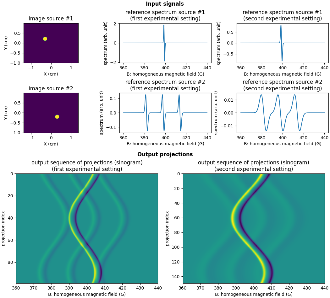
The two sinograms displayed above could also have been computed separately for each experiment but the ability of the projection operator to generate at once projections in multiple experimental settings means that it is also well suited to address inverse problems under this framework (i.e., when input projections come from various experimental conditions).

Multiple EPR sources (3D setting)

In this last section, we compute projection from multiple EPR sources in the three-dimensional setting. We use to that aim the function pyepri.multisrc.proj3d() that takes as input a sequence of 3D images of the individual paramagnetic species (one image per paramagnetic species present in the sample), the sequence of reference spectra of each individual paramagnetic species (one spectrum per paramagnetic species) and a sequence of 3D field gradient vector coordinates, it returns a sequence of 3D projections (3D sinogram) of the sample (mixture of paramagnetic species).

In the synthetic experiment performed below, we will use two EPR sources images, each one made of one ellipsoid. We will use a single line synthetic reference spectrum for the first source and a three lines synthetic reference spectrum for the second one. First, let us compute and display the 3D images of the two EPR sources.

# ---------------------------------------------------- #
# Compute a synthetic 3D images of the two EPR sources #
# ---------------------------------------------------- #

# compute sampling grids (the two sources images must share the same
# sampling step but can have different size, although we will use here
# the same size for both images)
Nx, Ny, Nz = 128, 256, 128 # image dimensions
delta = .02 # spatial sampling step (cm)
xgrid = (-(Nx//2) + backend.arange(Nx, dtype=dtype)) * delta
ygrid = (-(Ny//2) + backend.arange(Ny, dtype=dtype)) * delta
zgrid = (-(Nz//2) + backend.arange(Nz, dtype=dtype)) * delta
X, Y, Z = backend.meshgrid(xgrid, ygrid, zgrid)

# first source image (ellipsoid)
v_src1 = backend.cast(((X - .4) / .25)**2 + ((Y - .1) / .7)**2 + (((Z - .4) / .25)**2) <= 1., dtype=dtype)
v_src1 /= (delta**3 * v_src1.sum())

# second source image (another ellipsoid)
v_src2 = backend.cast(((X + .4) / .25)**2 + ((Y + .1) / .9)**2 + (((Z + .4) / .25)**2) <= 1., dtype=dtype)
v_src2 /= (delta**3 * v_src2.sum())

# ----------------------------------- #
# Display input 3D image (isosurface) #
# ----------------------------------- #

# compute isosurface sampling grid
grid = pv.StructuredGrid(backend.to_numpy(X), backend.to_numpy(Y), backend.to_numpy(Z))

# compute isosurface for the first source image
vol = np.moveaxis(backend.to_numpy(v_src1), (0,1,2), (2,1,0))
grid["vol"] = vol.flatten()
l1 = vol.max()
l0 = .2 * l1
isolevels = np.linspace(l0, l1, 10)
contours_src1 = grid.contour(isolevels)

# compute isosurface for the second source image
vol = np.moveaxis(backend.to_numpy(v_src2), (0,1,2), (2,1,0))
grid["vol"] = vol.flatten()
l1 = vol.max()
l0 = .2 * l1
isolevels = np.linspace(l0, l1, 10)
contours_src2 = grid.contour(isolevels)

# display isosurfaces
cpos = [(-3.8, 4.35, 2.11), (0.0, -0.1, 0.0), (-0.33, -0.62, 0.71)]
p = pv.Plotter()
p.camera_position = cpos
labels = dict(ztitle='Z', xtitle='X', ytitle='Y')
p.add_mesh(contours_src1, show_scalar_bar=False, color='#db0404', label=' source #1')
p.add_mesh(contours_src2, show_scalar_bar=False, color='#01b517', label=' source #2')
p.show_grid(**labels)
p.add_legend(face='r')
p.show()

Static Scene

Interactive Scene

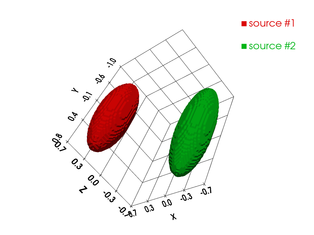
Next, let us compute and display the synthetic reference spectra of the two EPR sources as well as the field gradient orientations to use to generate the projections.

# ----------------------------------------------------------------- #
# Compute synthetic reference spectrum of the first EPR source (one #
# line spectrum)                                                    #
# ----------------------------------------------------------------- #
B = backend.linspace(360, 440, 1200, dtype=dtype)
Br1 = 399
sig1 = .36
cof1 = 1. / (sig1 * math.sqrt(2. * math.pi))
h1 = - cof1 * (B - Br1) / sig1**2 * backend.exp(- (B - Br1)**2 / (2. * sig1**2))

# -------------------------------------------------------------------- #
# Compute synthetic reference spectrum of the second EPR source (three #
# lines spectrum)                                                      #
# -------------------------------------------------------------------- #
Br2_left = 382
Br2_middle = 398
Br2_right = 414
sig2 = .8
cof2 = 1. / (3. * sig2 * math.sqrt(2. * math.pi))
h2_left = - cof2 * (B - Br2_left) / sig2**2 * backend.exp(- (B - Br2_left)**2 / (2. * sig2**2))
h2_middle = - cof2 * (B - Br2_middle) / sig2**2 * backend.exp(- (B - Br2_middle)**2 / (2. * sig2**2))
h2_right = - cof2 * (B - Br2_right) / sig2**2 * backend.exp(- (B - Br2_right)**2 / (2. * sig2**2))
h2 = h2_left + h2_middle + h2_right

# ------------------------------------------ #
# Compute field gradient vectors coordinates #
# ------------------------------------------ #
t1 = backend.linspace(0, 2. * math.pi, 32, dtype=dtype)
t2 = backend.linspace(0, 2. * math.pi, 32, dtype=dtype)
theta1, theta2 = backend.meshgrid(t1, t2)
theta1 = theta1.reshape((-1,)) # polar angles of the field gradients
theta2 = theta2.reshape((-1,)) # azimuthal angles of the field gradients
mu = 15 # field gradient amplitude (G/cm)
gx = mu * backend.cos(theta1) * backend.sin(theta2) # X-axis coordinates of the field gradient vectors
gy = mu * backend.sin(theta1) * backend.sin(theta2) # Y-axis coordinates of the field gradient vectors
gz = mu * backend.cos(theta2) # Z-axis coordinates of the field gradient vectors
fgrad = backend.stack((gx, gy, gz))

# ---------------------------------------------------- #
# Display reference spectra and field gradient vectors #
# ---------------------------------------------------- #

# reference spectrum of the first EPR source
fig = plt.figure(figsize=(15, 4.))
fig.add_subplot(1, 3, 1)
plt.plot(backend.to_numpy(B), backend.to_numpy(h1))
plt.grid(linestyle=':')
plt.xlabel('B: homogeneous magnetic field (G)')
plt.ylabel('spectrum (arb. unit)')
plt.title('reference spectrum source #1')

# reference spectrum of the second EPR source
fig.add_subplot(1, 3, 2)
plt.plot(backend.to_numpy(B), backend.to_numpy(h2))
plt.grid(linestyle=':')
plt.xlabel('B: homogeneous magnetic field (G)')
#plt.ylabel('spectrum (arb. unit)')
plt.title('reference spectrum source #2')

# magnetic field gradient vectors
ax = fig.add_subplot(1, 3, 3, projection='3d')
ax.scatter(backend.to_numpy(fgrad[0]), backend.to_numpy(fgrad[1]), backend.to_numpy(fgrad[2]))
ax.set_xlabel('X (cm)')
ax.set_ylabel('Y (cm)')
ax.set_zlabel('Z (cm)')
ax.set_aspect('equal', 'box')
_ = plt.title('magnetic field gradient samples')

Now we are ready to compute and display the projections of the mixture of EPR sources.

# ----------------------------------------------------- #
# Compute the projections of the mixture of EPR sources #
# ----------------------------------------------------- #
proj = multisrc.proj3d((v_src1, v_src2), delta, B, ((h1, h2),), (fgrad,), backend=backend)[0]

# -------------------------------- #
# Display the computed projections #
# -------------------------------- #
plt.figure(figsize=(8., 5.))
extent = (B[0].item(), B[-1].item(), proj.shape[0] - 1, 0)
plt.imshow(backend.to_numpy(proj), extent=extent, aspect='auto')
plt.xlabel('B: homogeneous magnetic field (G)')
plt.ylabel('projection index')
_ = plt.title('output sequence of projections (sinogram)')

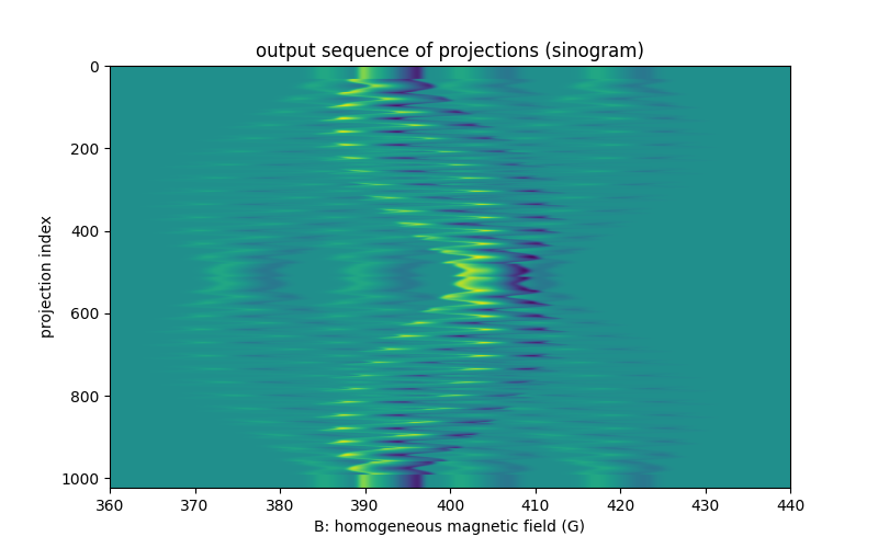
Remarks:

• As in the 2D setting, generating at once projections for multiple parameter settings is also possible in the 3D setting using the pyepri.multisrc.proj3d() operator.

• Again, the user must keep in mind that a large enough range for the input homogeneous magnetic field B is needed to generate realistic projections.

Next (backprojection): each projection operator presented here (may it be in the 2D or in the 3D setting, with single or multiple EPR source(s)) has an adjoint operator, usually referred as a backprojection operator. Fast and efficient implementations of those backprojection operators are available in the PyEPRI package. We encourage the reader to take a look at the dedicated backprojection tutorials.

Estimated memory usage: 513 MB