Embedded demonstration EPR datasets

Presentation of the EPR datasets embedded with this package.

We provide in this page some short descriptions of all demonstration EPR datasets embedded with the PyEPRI package (and used in the demonstration examples). We include load and display command line instructions. You can use the links listed below to jump to a specific dataset.

Two-dimensional EPR imaging datasets:

• irradiated phalanx (phalanx-20220203)

• Spade-Club-Diamond shapes printed with paramagnetic ink (scd-inkjet-20141204)

• Word “Bacteria” printed with paramagnetic ink (bacteria-inkjet-20100709)

• Word “CNRS” printed with paramagnetic ink (cnrs-inkjet-20110614)

• Mouse knee phantom (beads-phantom-20080313)

• Plastic beads in a thin tube filled with TAM (beads-thintubes-20081017)

• DPPH crystal powder in rubber (dpph-logo-20080402)

• Solutions of TAM & TEMPO in two distinct tubes (tam-and-tempo-tubes-2d-20210609)

Three-dimensional EPR imaging datasets:

• Fusillo soaked with 4OH-TEMPO (fusillo-20091002)

• TAM solution in tubes with various diameters (tamtubes-20211201)

• Solutions of TAM & TEMPO in two distinct tubes (tam-and-tempo-tubes-3d-20210609)

• TAM solution insert into a TEMPO solution (tam-insert-in-tempo-20230929)

Before presenting each dataset, let us prepare the data loading process.

# --------------------- #
# Import needed modules #
# --------------------- #
import numpy as np # for array manipulations
import matplotlib.pyplot as plt # tools for data visualization
import pyepri.backends as backends # to instanciate PyEPRI backends
import pyepri.datasets as datasets # to retrieve the path (on your own machine) of the demo dataset
import pyepri.io as io # tools for loading EPR datasets (in BES3T or Python .PKL format)
plt.ion()

# -------------- #
# Create backend #
# -------------- #
#
# We create a numpy backend here because it should be available on
# your system (as a mandatory dependency of the PyEPRI
# package).
#
# However, you can also try another backend (if available on your
# system) by uncommenting one of the following commands. Depending on
# your system, using another backend may drastically reduce the
# computation time in practical applications.
#
backend = backends.create_numpy_backend()
#backend = backends.create_torch_backend('cpu') # uncomment here for torch-cpu backend
#backend = backends.create_cupy_backend() # uncomment here for cupy backend
#backend = backends.create_torch_backend('cuda') # uncomment here for torch-gpu backend

Irradiated phalanx (2D)

The sample is an irradiated distal phalanx. It was kindly provided to LCBPT by our colleague Pr. Bernard Gallez (UC Louvain).

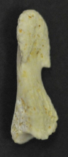
Irradiations generate paramagnetic damages of the bone lattice microarchitecture that can be observed using EPR imaging.

The dataset was acquired at LCBPT using an X-band Bruker spectrometer. It comprised of two files in .pkl format:

• phalanx-20220203-h.pkl: contains the reference spectrum (1D spectrum) of the sample and the associated homogeneous magnetic field intensity (sampling nodes);

• phalanx-20220203-proj.pkl: contains the 2D projections (= 2D sinogram), the associated homogeneous magnetic field intensity nodes and the corresponding field gradient vectors coordinates.

The dataset contains 113 projections acquired with constant field gradient magnitude equal to 168 G/cm and orientation uniformly sampled between 0 and 180°. Each projection contains 2000 measurement points (same for the reference spectrum). The next commands show how to open and display the dataset.

#--------------#
# Load dataset #
#--------------#
dtype = 'float32'
path_proj = datasets.get_path('phalanx-20220203-proj.pkl') # returns the location of this dataset on your system
path_h = datasets.get_path('phalanx-20220203-h.pkl') # returns the location of this dataset on your system
dataset_proj = io.load(path_proj, backend=backend, dtype=dtype) # load the dataset containing the projections
dataset_h = io.load(path_h, backend=backend, dtype=dtype) # load the dataset containing the reference spectrum
B = dataset_proj['B'] # get B nodes from the loaded dataset
proj = dataset_proj['DAT'] # get projections data from the loaded dataset
fgrad = dataset_proj['FGRAD'] # get field gradient data from the loaded dataset
h = dataset_h['DAT'] # get reference spectrum data from the loaded dataset

# ------------------------------------------------------------ #
# Compute and display several important acquisition parameters #
# ------------------------------------------------------------ #
print("Sweep-width = %g G" % (B[-1] - B[0]))
print("Number of projections = %d" % proj.shape[0])
print("Number of point per projection = %d" % proj.shape[1])
mu = backend.sqrt(fgrad[0]**2 + fgrad[1]**2) # magnitudes of the field gradient vectors (constant for this dataset)
print("Field gradient magnitude = %g G/cm" % mu[0])

#-----------------#
# Display dataset #
#-----------------#

# display the reference spectrum
plt.figure(figsize=(13, 5))
plt.subplot(1, 2, 1)
plt.plot(backend.to_numpy(B), backend.to_numpy(h))
plt.xlabel('B: homogeneous magnetic field intensity (G)')
plt.ylabel('measurements (arb. units)')
plt.title('reference spectrum (h)')

# display the field gradient vector associated to the measured projections
plt.subplot(1, 2, 2)
plt.plot(backend.to_numpy(fgrad[0]), backend.to_numpy(fgrad[1]), 'go', markersize=1)
plt.gca().set_aspect('equal')
plt.xlabel("horizontal axis (G/cm)")
plt.ylabel("vertical axis (G/cm)")
_ = plt.title("2D field gradient vectors")

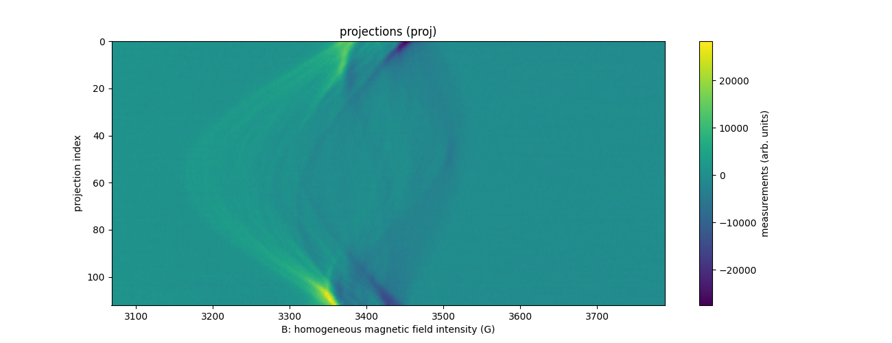
# display the projections
plt.figure(figsize=(13, 5))
extent = (B[0].item(), B[-1].item(), proj.shape[0] - 1, 0)
plt.imshow(backend.to_numpy(proj), extent=extent, aspect='auto')
cbar = plt.colorbar()
cbar.set_label('measurements (arb. units)')
plt.xlabel('B: homogeneous magnetic field intensity (G)')
plt.ylabel('projection index')
_ = plt.title('projections (proj)')

• 
• 

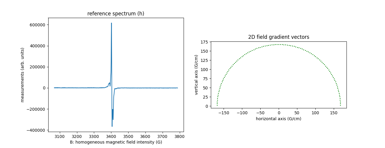
Sweep-width = 719.44 G
Number of projections = 113
Number of point per projection = 2000
Field gradient magnitude = 168 G/cm

Note: this dataset is also available in ASCII format (files phalanx-20220203-h.txt, phalanx-20220203-proj.txt, phalanx-20220203-fgrad.txt, phalanx-20220203-B.txt) and in the original BES3T format (files phalanx-20220203-h.DTA, phalanx-20220203-h.DSC, phalanx-20220203-proj.DTA and phalanx-20220203-proj.DSC). See here how to deal with those kinds of files.

Paramagnetic ink (2D)

The three next datasets correspond to paramagnetic ink printed on paper sheets.

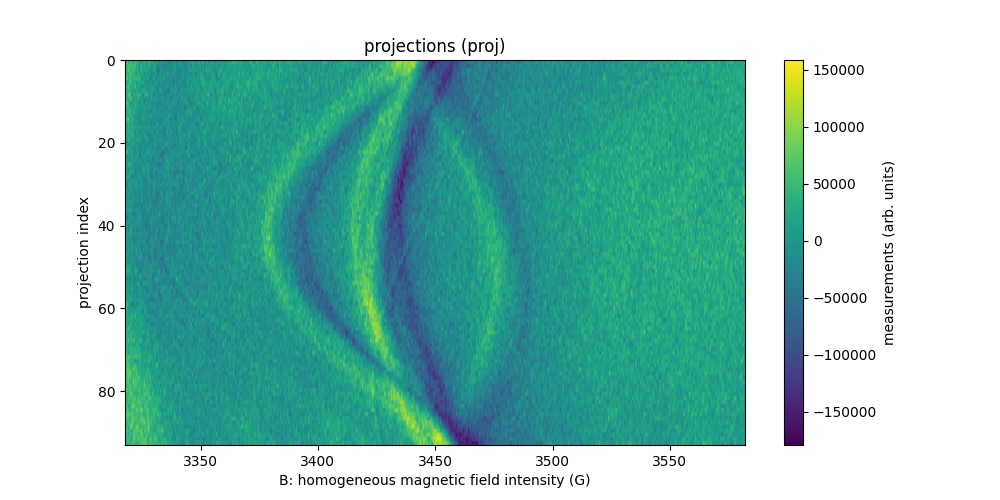
Spade-Club-Diamond shapes printed on a paper sheet

We present below the scd-inkjet-20141204 dataset, acquired at LCBPT using an X-band Bruker spectrometer.

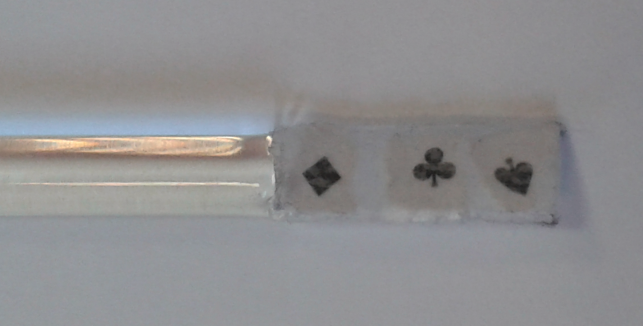
The dataset is comprised of .pkl files stored using the same suffix naming conventions as the other datasets (datasetname-{proj,h}.npy). It contains 94 projections acquired with constant field gradient magnitude equal to 57.6 G/cm and orientation uniformly sampled between -90° and 90°. Each projection contains 1300 measurement points (same for the reference spectrum). The next commands show how to open and display the dataset.

#--------------#
# Load dataset #
#--------------#
dtype = 'float32'
datasetname = 'scd-inkjet-20141204'
path_proj = datasets.get_path(datasetname + '-proj.pkl') # returns the location of this dataset on your system
path_h = datasets.get_path(datasetname + '-h.pkl') # returns the location of this dataset on your system
dataset_proj = io.load(path_proj, backend=backend, dtype=dtype) # load the dataset containing the projections
dataset_h = io.load(path_h, backend=backend, dtype=dtype) # load the dataset containing the reference spectrum
B = dataset_proj['B'] # get B nodes from the loaded dataset
proj = dataset_proj['DAT'] # get projections data from the loaded dataset
fgrad = dataset_proj['FGRAD'] # get field gradient data from the loaded dataset
h = dataset_h['DAT'] # get reference spectrum data from the loaded dataset

# ------------------------------------------------------------ #
# Compute and display several important acquisition parameters #
# ------------------------------------------------------------ #
print("Sweep-width = %g G" % (B[-1] - B[0]))
print("Number of projections = %d" % proj.shape[0])
print("Number of point per projection = %d" % proj.shape[1])
mu = backend.sqrt(fgrad[0]**2 + fgrad[1]**2) # magnitudes of the field gradient vectors (constant for this dataset)
print("Field gradient magnitude = %g G/cm" % mu[0])

#-----------------#
# Display dataset #
#-----------------#

# display the reference spectrum
plt.figure(figsize=(15, 5))
plt.suptitle("Dataset '" + datasetname + "'",  weight='demibold');
plt.subplot(1, 2, 1)
plt.plot(backend.to_numpy(B), backend.to_numpy(h))
plt.xlabel('B: homogeneous magnetic field intensity (G)')
plt.ylabel('measurements (arb. units)')
plt.title('reference spectrum (h)')

# display the field gradient vector associated to the measured projections
plt.subplot(1, 2, 2)
plt.plot(backend.to_numpy(fgrad[0]), backend.to_numpy(fgrad[1]), 'go', markersize=1)
plt.gca().set_aspect('equal')
plt.xlabel("horizontal axis (G/cm)")
plt.ylabel("vertical axis (G/cm)")
_ = plt.title("2D field gradient vectors")

# display the projections
plt.figure(figsize=(10, 5))
extent = (B[0].item(), B[-1].item(), proj.shape[0] - 1, 0)
plt.imshow(backend.to_numpy(proj), extent=extent, aspect='auto')
cbar = plt.colorbar()
cbar.set_label('measurements (arb. units)')
plt.xlabel('B: homogeneous magnetic field intensity (G)')
plt.ylabel('projection index')
_ = plt.title('projections (proj)')

• 
• 

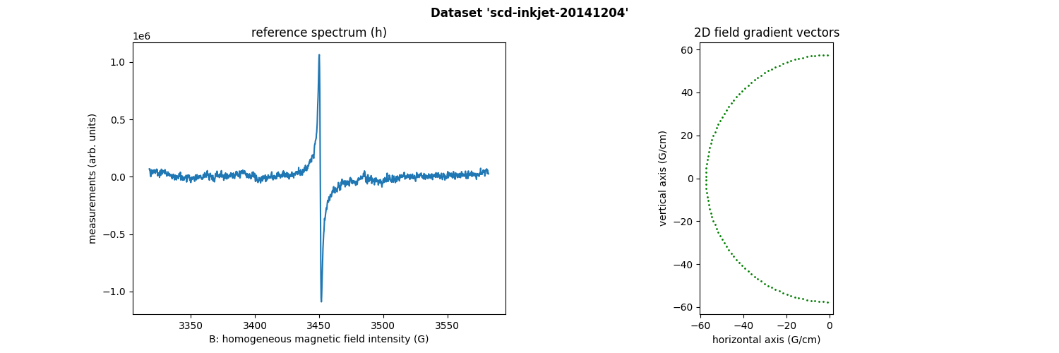
Sweep-width = 264.197 G
Number of projections = 94
Number of point per projection = 1300
Field gradient magnitude = 57.6 G/cm

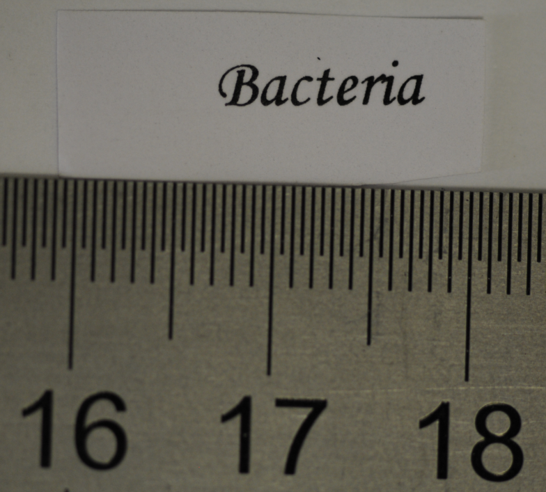
Word “Bacteria” printed on a paper sheet

Here is the bacteria-inkjet-20100709 dataset, acquired at LCBPT using an X-band Bruker spectrometer.

#--------------#
# Load dataset #
#--------------#
dtype = 'float32'
datasetname = 'bacteria-inkjet-20100709'
path_proj = datasets.get_path(datasetname + '-proj.pkl') # returns the location of this dataset on your system
path_h = datasets.get_path(datasetname + '-h.pkl') # returns the location of this dataset on your system
dataset_proj = io.load(path_proj, backend=backend, dtype=dtype) # load the dataset containing the projections
dataset_h = io.load(path_h, backend=backend, dtype=dtype) # load the dataset containing the reference spectrum
B = dataset_proj['B'] # get B nodes from the loaded dataset
proj = dataset_proj['DAT'] # get projections data from the loaded dataset
fgrad = dataset_proj['FGRAD'] # get field gradient data from the loaded dataset
h = dataset_h['DAT'] # get reference spectrum data from the loaded dataset

# ------------------------------------------------------------ #
# Compute and display several important acquisition parameters #
# ------------------------------------------------------------ #
print("Sweep-width = %g G" % (B[-1] - B[0]))
print("Number of projections = %d" % proj.shape[0])
print("Number of point per projection = %d" % proj.shape[1])
mu = backend.sqrt(fgrad[0]**2 + fgrad[1]**2) # magnitudes of the field gradient vectors (constant for this dataset)
print("Field gradient magnitude = %g G/cm" % mu[0])

#-----------------#
# Display dataset #
#-----------------#

# display the reference spectrum
plt.figure(figsize=(10, 5))
plt.suptitle("Dataset '" + datasetname + "'",  weight='demibold');
plt.subplot(1, 2, 1)
plt.plot(backend.to_numpy(B), backend.to_numpy(h))
plt.xlabel('B: homogeneous magnetic field intensity (G)')
plt.ylabel('measurements (arb. units)')
plt.title('reference spectrum (h)')

# display the projections
plt.subplot(1, 2, 2)
plt.plot(backend.to_numpy(fgrad[0]), backend.to_numpy(fgrad[1]), 'go', markersize=1)
plt.gca().set_aspect('equal')
plt.xlabel("horizontal axis (G/cm)")
plt.ylabel("vertical axis (G/cm)")
_ = plt.title("2D field gradient vectors")

# display the field gradient vector associated to the measured projections
plt.figure(figsize=(10, 5))
extent = (B[0].item(), B[-1].item(), proj.shape[0] - 1, 0)
plt.imshow(backend.to_numpy(proj), extent=extent, aspect='auto')
cbar = plt.colorbar()
cbar.set_label('measurements (arb. units)')
plt.xlabel('B: homogeneous magnetic field intensity (G)')
plt.ylabel('projection index')
_ = plt.title('projections (proj)')

• 
• 

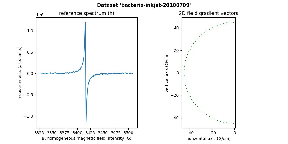
Sweep-width = 180.646 G
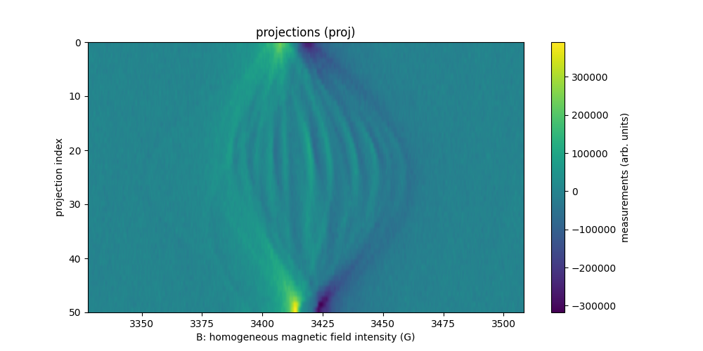
Number of projections = 51
Number of point per projection = 512
Field gradient magnitude = 45 G/cm

Word “CNRS” printed on a paper sheet

The last dataset of this series of printed paramagnetic ink is the cnrs-inkjet-20110614 dataset, acquired at LCBPT using an X-band Bruker spectrometer. The sample is a sheet of paper on which the word “CNRS” is printed with paramagnetic ink. Unfortunately no picture of the sample is currently available.

#--------------#
# Load dataset #
#--------------#
dtype = 'float32'
datasetname = 'cnrs-inkjet-20110614'
path_proj = datasets.get_path(datasetname + '-proj.pkl') # returns the location of this dataset on your system
path_h = datasets.get_path(datasetname + '-h.pkl') # returns the location of this dataset on your system
dataset_proj = io.load(path_proj, backend=backend, dtype=dtype) # load the dataset containing the projections
dataset_h = io.load(path_h, backend=backend, dtype=dtype) # load the dataset containing the reference spectrum
B = dataset_proj['B'] # get B nodes from the loaded dataset
proj = dataset_proj['DAT'] # get projections data from the loaded dataset
fgrad = dataset_proj['FGRAD'] # get field gradient data from the loaded dataset
h = dataset_h['DAT'] # get reference spectrum data from the loaded dataset

# ------------------------------------------------------------ #
# Compute and display several important acquisition parameters #
# ------------------------------------------------------------ #
print("Sweep-width = %g G" % (B[-1] - B[0]))
print("Number of projections = %d" % proj.shape[0])
print("Number of point per projection = %d" % proj.shape[1])
mu = backend.sqrt(fgrad[0]**2 + fgrad[1]**2) # magnitudes of the field gradient vectors (constant for this dataset)
print("Field gradient magnitude = %g G/cm" % mu[0])

#-----------------#
# Display dataset #
#-----------------#

# display the reference spectrum
plt.figure(figsize=(10, 5))
plt.suptitle("Dataset '" + datasetname + "'",  weight='demibold');
plt.subplot(1, 2, 1)
plt.plot(backend.to_numpy(B), backend.to_numpy(h))
plt.xlabel('B: homogeneous magnetic field intensity (G)')
plt.ylabel('measurements (arb. units)')
plt.title('reference spectrum (h)')

# display the projections
plt.subplot(1, 2, 2)
plt.plot(backend.to_numpy(fgrad[0]), backend.to_numpy(fgrad[1]), 'go', markersize=1)
plt.gca().set_aspect('equal')
plt.xlabel("horizontal axis (G/cm)")
plt.ylabel("vertical axis (G/cm)")
_ = plt.title("2D field gradient vectors")

# display the field gradient vector associated to the measured projections
plt.figure(figsize=(10, 5))
extent = (B[0].item(), B[-1].item(), proj.shape[0] - 1, 0)
im_hdl = plt.imshow(backend.to_numpy(proj), extent=extent, aspect='auto')
cmax = backend.quantile(proj, .9995)
im_hdl.set_clim(proj.min().item(), cmax.item()) # saturate 0.05% of the highest values
cbar = plt.colorbar()
cbar.set_label('measurements (arb. units)')
plt.xlabel('B: homogeneous magnetic field intensity (G)')
plt.ylabel('projection index')
_ = plt.title('projections (proj)\n(saturation of 0.05% of the max. values)')

• 
• 

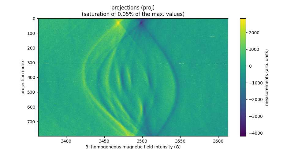
Sweep-width = 249.5 G
Number of projections = 800
Number of point per projection = 1024
Field gradient magnitude = 175 G/cm

Plastic beads in TAM solution (2D)

The two next datasets are made of plastic beads placed in a tube filled with a solution of TAM.

Mouse knee phantom (2D)

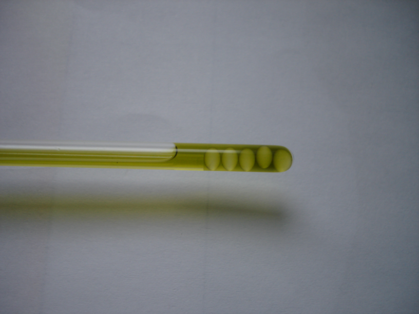
The sample in the beads-phantom-20080313 dataset is made of a single EPR tube (with 3 mm internal diameter) containing plastic beads with diameter 2.5 mm and a TAM aqueous solution with concentration 5 mM. The sample has been designed to represent a mouse knee phantom.

This beads-phantom-20080313`` dataset has been acquired at LCBPT using an L-band Bruker spectrometer.

#--------------#
# Load dataset #
#--------------#
dtype = 'float32'
datasetname = 'beads-phantom-20080313'
path_proj = datasets.get_path(datasetname + '-proj.pkl') # returns the location of this dataset on your system
path_h = datasets.get_path(datasetname + '-h.pkl') # returns the location of this dataset on your system
dataset_proj = io.load(path_proj, backend=backend, dtype=dtype) # load the dataset containing the projections
dataset_h = io.load(path_h, backend=backend, dtype=dtype) # load the dataset containing the reference spectrum
B = dataset_proj['B'] # get B nodes from the loaded dataset
proj = dataset_proj['DAT'] # get projections data from the loaded dataset
fgrad = dataset_proj['FGRAD'] # get field gradient data from the loaded dataset
h = dataset_h['DAT'] # get reference spectrum data from the loaded dataset

# ------------------------------------------------------------ #
# Compute and display several important acquisition parameters #
# ------------------------------------------------------------ #
print("Sweep-width = %g G" % (B[-1] - B[0]))
print("Number of projections = %d" % proj.shape[0])
print("Number of point per projection = %d" % proj.shape[1])
mu = backend.sqrt(fgrad[0]**2 + fgrad[1]**2) # magnitudes of the field gradient vectors (constant for this dataset)
print("Field gradient magnitude = %g G/cm" % mu[0])

#-----------------#
# Display dataset #
#-----------------#

# display the reference spectrum
plt.figure(figsize=(10, 5))
plt.suptitle("Dataset '" + datasetname + "'",  weight='demibold');
plt.subplot(1, 2, 1)
plt.plot(backend.to_numpy(B), backend.to_numpy(h))
plt.xlabel('B: homogeneous magnetic field intensity (G)')
plt.ylabel('measurements (arb. units)')
plt.title('reference spectrum (h)')

# display the projections
plt.subplot(1, 2, 2)
plt.plot(backend.to_numpy(fgrad[0]), backend.to_numpy(fgrad[1]), 'go', markersize=1)
plt.gca().set_aspect('equal')
plt.xlabel("horizontal axis (G/cm)")
plt.ylabel("vertical axis (G/cm)")
_ = plt.title("2D field gradient vectors")

# display the field gradient vector associated to the measured projections
plt.figure(figsize=(10, 5))
extent = (B[0].item(), B[-1].item(), proj.shape[0] - 1, 0)
plt.imshow(backend.to_numpy(proj), extent=extent, aspect='auto')
cbar = plt.colorbar()
cbar.set_label('measurements (arb. units)')
plt.xlabel('B: homogeneous magnetic field intensity (G)')
plt.ylabel('projection index')
_ = plt.title('projections (proj)')

• 
• 

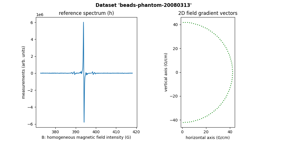
Sweep-width = 45.5555 G
Number of projections = 76
Number of point per projection = 1024
Field gradient magnitude = 42.04 G/cm

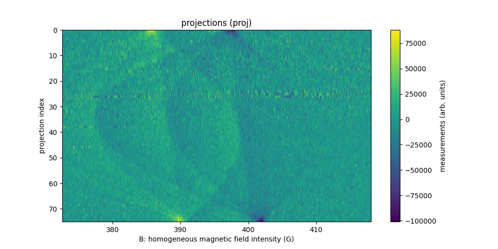
Plastic beads in a thin tube (2D)

The sample in the beads-thintubes-20081017 dataset is made of a single capillary tube with 0.5 mm diameter containing TAM aqueous solution with concentration 5 mM and some plastic beads with 0.4 mm diameter.

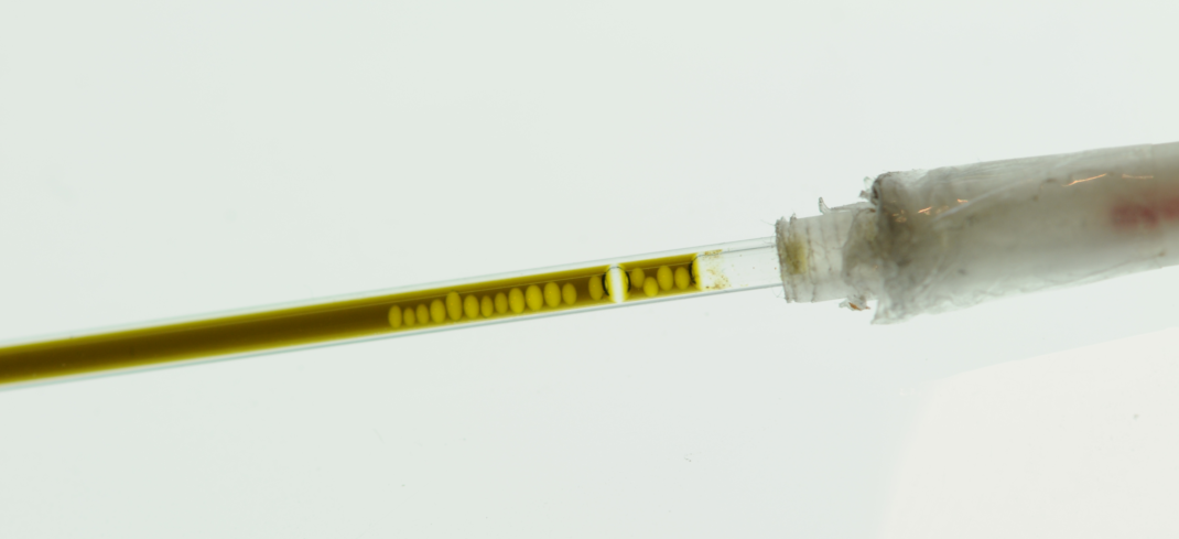
This beads-thintubes-20081017 dataset has been acquired at LCBPT using an X-band Bruker spectrometer .

#--------------#
# Load dataset #
#--------------#
dtype = 'float32'
datasetname = 'beads-thintubes-20081017'
path_proj = datasets.get_path(datasetname + '-proj.pkl') # returns the location of this dataset on your system
path_h = datasets.get_path(datasetname + '-h.pkl') # returns the location of this dataset on your system
dataset_proj = io.load(path_proj, backend=backend, dtype=dtype) # load the dataset containing the projections
dataset_h = io.load(path_h, backend=backend, dtype=dtype) # load the dataset containing the reference spectrum
B = dataset_proj['B'] # get B nodes from the loaded dataset
proj = dataset_proj['DAT'] # get projections data from the loaded dataset
fgrad = dataset_proj['FGRAD'] # get field gradient data from the loaded dataset
h = dataset_h['DAT'] # get reference spectrum data from the loaded dataset

# ------------------------------------------------------------ #
# Compute and display several important acquisition parameters #
# ------------------------------------------------------------ #
print("Sweep-width = %g G" % (B[-1] - B[0]))
print("Number of projections = %d" % proj.shape[0])
print("Number of point per projection = %d" % proj.shape[1])
mu = backend.sqrt(fgrad[0]**2 + fgrad[1]**2) # magnitudes of the field gradient vectors (constant for this dataset)
print("Field gradient magnitude = %g G/cm" % mu[0])

#-----------------#
# Display dataset #
#-----------------#

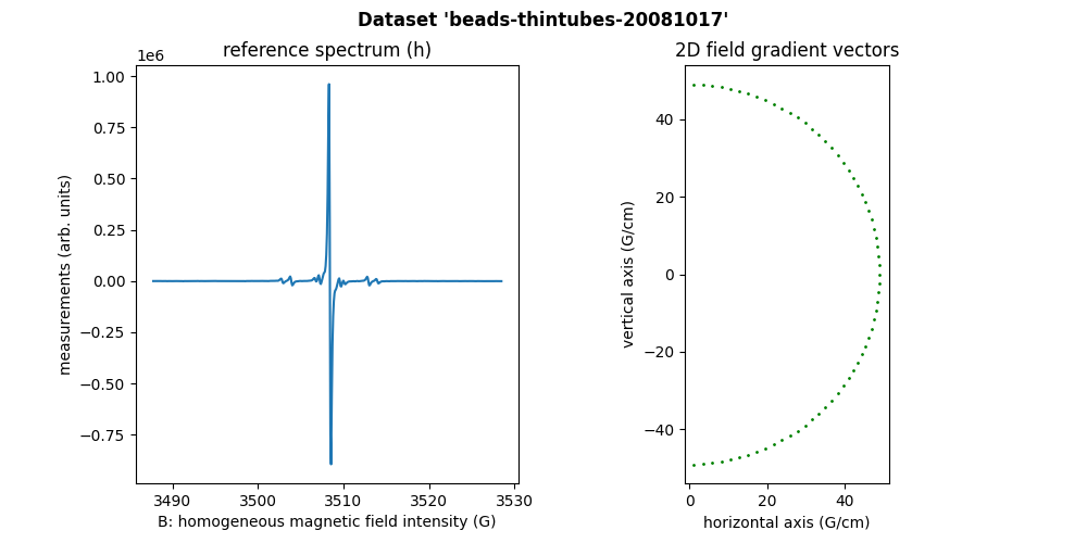
# display the reference spectrum
plt.figure(figsize=(10, 5))
plt.suptitle("Dataset '" + datasetname + "'",  weight='demibold');
plt.subplot(1, 2, 1)
plt.plot(backend.to_numpy(B), backend.to_numpy(h))
plt.xlabel('B: homogeneous magnetic field intensity (G)')
plt.ylabel('measurements (arb. units)')
plt.title('reference spectrum (h)')


# display the projections
plt.subplot(1, 2, 2)
plt.plot(backend.to_numpy(fgrad[0]), backend.to_numpy(fgrad[1]), 'go', markersize=1)
plt.gca().set_aspect('equal')
plt.xlabel("horizontal axis (G/cm)")
plt.ylabel("vertical axis (G/cm)")
_ = plt.title("2D field gradient vectors")

# display the field gradient vector associated to the measured projections
plt.figure(figsize=(10, 5))
extent = (B[0].item(), B[-1].item(), proj.shape[0] - 1, 0)
im_hdl = plt.imshow(backend.to_numpy(proj), extent=extent, aspect='auto')
cmin = backend.quantile(proj, .005)
cmax = backend.quantile(proj, .995)
im_hdl.set_clim(cmin.item(), cmax.item()) # saturate .5% of the lowest and highest values
cbar = plt.colorbar()
cbar.set_label('measurements (arb. units)')
plt.xlabel('B: homogeneous magnetic field intensity (G)')
plt.ylabel('projection index')
_ = plt.title('projections (proj)\n(saturation of 0.5% of the min/max values)')

• 
• 

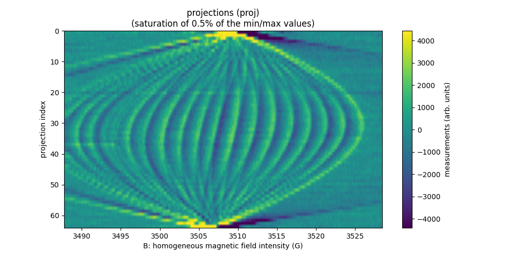
Sweep-width = 40.7202 G
Number of projections = 65
Number of point per projection = 512
Field gradient magnitude = 49 G/cm

DPPH cristal powder in rubber (2D)

The (former) CNRS logo has been engraved in rubber, then filled with DDPH powder.

Then, the dpph-logo-20080402 dataset has been acquired at LCBPT using an L-band Bruker spectrometer .

#--------------#
# Load dataset #
#--------------#
dtype = 'float32'
datasetname = 'dpph-logo-20080402'
path_proj = datasets.get_path(datasetname + '-proj.pkl') # returns the location of this dataset on your system
path_h = datasets.get_path(datasetname + '-h.pkl') # returns the location of this dataset on your system
dataset_proj = io.load(path_proj, backend=backend, dtype=dtype) # load the dataset containing the projections
dataset_h = io.load(path_h, backend=backend, dtype=dtype) # load the dataset containing the reference spectrum
B = dataset_proj['B'] # get B nodes from the loaded dataset
proj = dataset_proj['DAT'] # get projections data from the loaded dataset
fgrad = dataset_proj['FGRAD'] # get field gradient data from the loaded dataset
h = dataset_h['DAT'] # get reference spectrum data from the loaded dataset

# ------------------------------------------------------------ #
# Compute and display several important acquisition parameters #
# ------------------------------------------------------------ #
print("Sweep-width = %g G" % (B[-1] - B[0]))
print("Number of projections = %d" % proj.shape[0])
print("Number of point per projection = %d" % proj.shape[1])
mu = backend.sqrt(fgrad[0]**2 + fgrad[1]**2) # magnitudes of the field gradient vectors (constant for this dataset)
print("Field gradient magnitude = %g G/cm" % mu[0])

#-----------------#
# Display dataset #
#-----------------#

# display the reference spectrum
plt.figure(figsize=(10, 5))
plt.suptitle("Dataset '" + datasetname + "'",  weight='demibold');
plt.subplot(1, 2, 1)
plt.plot(backend.to_numpy(B), backend.to_numpy(h))
plt.xlabel('B: homogeneous magnetic field intensity (G)')
plt.ylabel('measurements (arb. units)')
plt.title('reference spectrum (h)')

# display the field gradient vector associated to the measured projections
plt.subplot(1, 2, 2)
plt.plot(backend.to_numpy(fgrad[0]), backend.to_numpy(fgrad[1]), 'go', markersize=1)
plt.gca().set_aspect('equal')
plt.xlabel("horizontal axis (G/cm)")
plt.ylabel("vertical axis (G/cm)")
_ = plt.title("2D field gradient vectors")

# display the projections
plt.figure(figsize=(10, 5))
extent = (B[0].item(), B[-1].item(), proj.shape[0] - 1, 0)
im_hdl = plt.imshow(backend.to_numpy(proj), extent=extent, aspect='auto')
cbar = plt.colorbar()
cbar.set_label('measurements (arb. units)')
plt.xlabel('B: homogeneous magnetic field intensity (G)')
plt.ylabel('projection index')
_ = plt.title('projections (proj)')

• 
• 

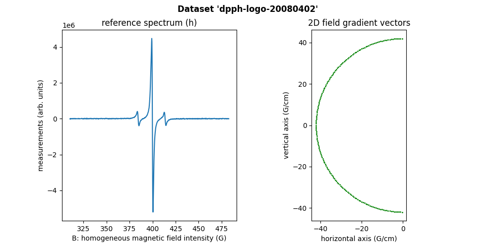
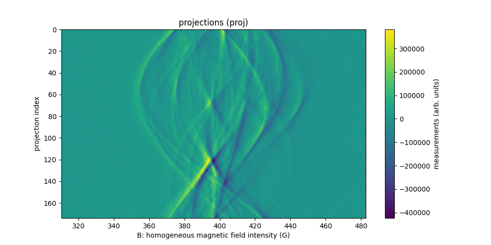
Sweep-width = 172.531 G
Number of projections = 175
Number of point per projection = 1024
Field gradient magnitude = 42.04 G/cm

Fusillo soaked with TEMPO (3D)

The next sample is made of a fusillo with helical shape which was put into a 4 mM aqueous solution of 4OH-TEMPO for a night, then dried using paper.

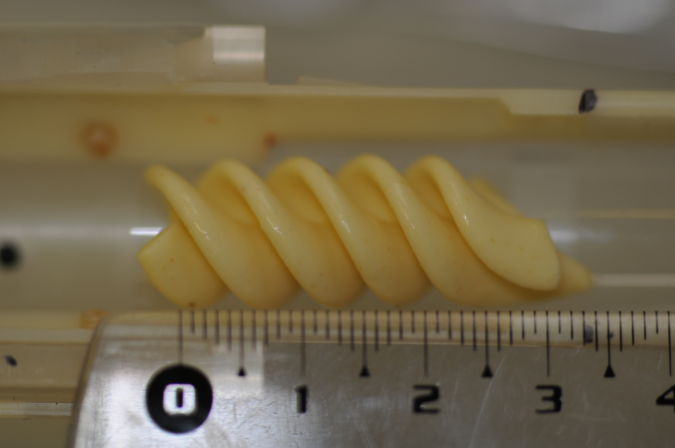
The dataset fusillo-20091002 is three dimensional and has been acquired at LCBPT using an L-band Bruker spectrometer.

#--------------#
# Load dataset #
#--------------#
dtype = 'float32'
datasetname = 'fusillo-20091002'
path_proj = datasets.get_path(datasetname + '-proj.pkl') # returns the location of this dataset on your system
path_h = datasets.get_path(datasetname + '-h.pkl') # returns the location of this dataset on your system
dataset_proj = io.load(path_proj, backend=backend, dtype=dtype) # load the dataset containing the projections
dataset_h = io.load(path_h, backend=backend, dtype=dtype) # load the dataset containing the reference spectrum
B = dataset_proj['B'] # get B nodes from the loaded dataset
proj = dataset_proj['DAT'] # get projections data from the loaded dataset
fgrad = dataset_proj['FGRAD'] # get field gradient data from the loaded dataset
h = dataset_h['DAT'] # get reference spectrum data from the loaded dataset

# ------------------------------------------------------------ #
# Compute and display several important acquisition parameters #
# ------------------------------------------------------------ #
print("Sweep-width = %g G" % (B[-1] - B[0]))
print("Number of projections = %d" % proj.shape[0])
print("Number of point per projection = %d" % proj.shape[1])
mu = backend.sqrt(fgrad[0]**2 + fgrad[1]**2 + fgrad[2]**2) # magnitudes of the field gradient vectors (constant for this dataset)
print("Field gradient magnitude = %g G/cm" % mu[0])

#-----------------#
# Display dataset #
#-----------------#

# display the reference spectrum
fig = plt.figure(figsize=(10, 5))
fig.add_subplot(1, 2, 1)
plt.plot(backend.to_numpy(B), backend.to_numpy(h))
plt.grid(linestyle=':')
plt.xlabel('B: homogeneous magnetic field intensity (G)')
plt.ylabel('measurements (arb. units)')
plt.title('reference spectrum (h)')
plt.suptitle("Dataset '" + datasetname + "'",  weight='demibold');

# display the field gradient vector associated to the measured projections
ax = fig.add_subplot(1, 2, 2, projection='3d')
ax.scatter(backend.to_numpy(fgrad[0]), backend.to_numpy(fgrad[1]), backend.to_numpy(fgrad[2]))
ax.set_xlim(-15, 15)
ax.set_ylim(-15, 15)
ax.set_zlim(-15, 15)
ax.set_aspect('equal', 'box')
ax.set_xlabel("X axis (G/cm)")
ax.set_ylabel("Y axis (G/cm)")
ax.set_zlabel("Z axis (G/cm)")
_ = plt.title('magnetic field gradient samples')

# display the projections
plt.figure(figsize=(10, 5))
extent = (B[0].item(), B[-1].item(), proj.shape[0] - 1, 0)
im_hdl = plt.imshow(backend.to_numpy(proj), extent=extent, aspect='auto')
cbar = plt.colorbar()
cbar.set_label('measurements (arb. units)')
plt.xlabel('B: homogeneous magnetic field intensity (G)')
plt.ylabel('projection index')
_ = plt.title('projections (proj)')

• 
• 

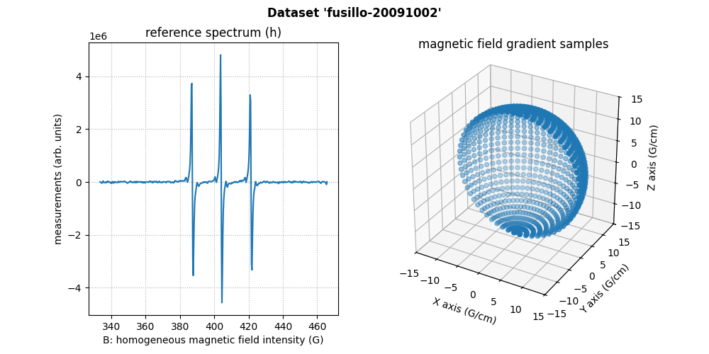
Sweep-width = 132.235 G
Number of projections = 961
Number of point per projection = 500
Field gradient magnitude = 14 G/cm

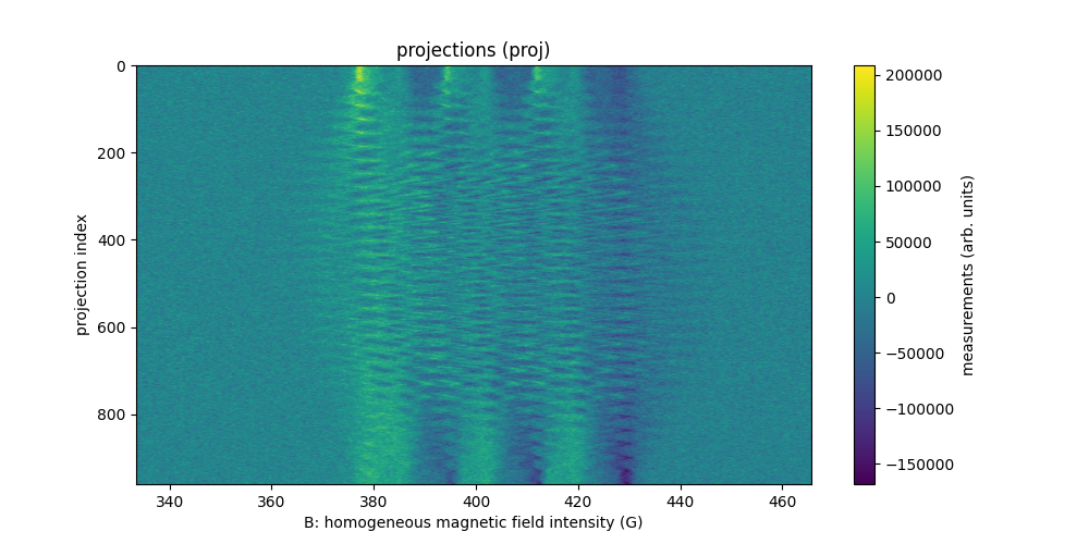
TAM solution in tubes with various diameters (3D)

The sample is made of six capillary tubes filled with an aqueous TAM solution with concentration 1 mM. The tubes were sealed using wax sealed plate (Fischer scientific) and attached together using masking tape.

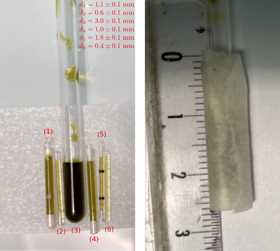
The dataset tamtubes-20211201 is three dimensional and has been acquired at LCBPT using an L-band Bruker spectrometer.

Important: it should be noted that tubes (1) and (6) were badly sealed and leaked (partially for tube (1) and totally for tube (6)) during the experiment.

#--------------#
# Load dataset #
#--------------#
dtype = 'float32'
datasetname = 'tamtubes-20211201'
path_proj = datasets.get_path(datasetname + '-proj.pkl') # returns the location of this dataset on your system
path_h = datasets.get_path(datasetname + '-h.pkl') # returns the location of this dataset on your system
dataset_proj = io.load(path_proj, backend=backend, dtype=dtype) # load the dataset containing the projections
dataset_h = io.load(path_h, backend=backend, dtype=dtype) # load the dataset containing the reference spectrum
B = dataset_proj['B'] # get B nodes from the loaded dataset
proj = dataset_proj['DAT'] # get projections data from the loaded dataset
fgrad = dataset_proj['FGRAD'] # get field gradient data from the loaded dataset
h = dataset_h['DAT'] # get reference spectrum data from the loaded dataset

# ------------------------------------------------------------ #
# Compute and display several important acquisition parameters #
# ------------------------------------------------------------ #
print("Sweep-width = %g G" % (B[-1] - B[0]))
print("Number of projections = %d" % proj.shape[0])
print("Number of point per projection = %d" % proj.shape[1])
mu = backend.sqrt(fgrad[0]**2 + fgrad[1]**2 + fgrad[2]**2) # magnitudes of the field gradient vectors (constant for this dataset)
print("Field gradient magnitude = %g G/cm" % mu[0])

#-----------------#
# Display dataset #
#-----------------#

# display the reference spectrum
fig = plt.figure(figsize=(19, 9))
ax = fig.add_subplot(1, 2, 1)
plt.plot(backend.to_numpy(B), backend.to_numpy(h))
plt.grid(linestyle=':')
plt.xlabel('B: homogeneous magnetic field intensity (G)')
plt.ylabel('measurements (arb. units)')
plt.title('reference spectrum (h)')
plt.suptitle("Dataset '" + datasetname + "'",  weight='demibold', fontsize=20);
for item in ([ax.title, ax.xaxis.label, ax.yaxis.label] +
             ax.get_xticklabels() + ax.get_yticklabels()):
    item.set_fontsize(16)

# display the field gradient vector associated to the measured projections
ax = fig.add_subplot(1, 2, 2, projection='3d')
ax.scatter(backend.to_numpy(fgrad[0]), backend.to_numpy(fgrad[1]), backend.to_numpy(fgrad[2]))
ax.set_xlim(-15, 15)
ax.set_ylim(-15, 15)
ax.set_zlim(-15, 15)
ax.set_aspect('equal', 'box')
ax.set_xlabel("X axis (G/cm)")
ax.set_ylabel("Y axis (G/cm)")
ax.set_zlabel("Z axis (G/cm)")
_ = plt.title('magnetic field gradient samples')
for item in ([ax.title, ax.xaxis.label, ax.yaxis.label,
              ax.zaxis.label] + ax.get_xticklabels() +
             ax.get_yticklabels() + ax.get_zticklabels()):
    item.set_fontsize(16)

# display the projections
plt.figure(figsize=(10, 5))
extent = (B[0].item(), B[-1].item(), proj.shape[0] - 1, 0)
im_hdl = plt.imshow(backend.to_numpy(proj), extent=extent, aspect='auto')
cmin = backend.quantile(proj, .001)
cmax = backend.quantile(proj, .999)
im_hdl.set_clim(cmin.item(), cmax.item()) # saturate 0.1% of the highest values
cbar = plt.colorbar()
cbar.set_label('measurements (arb. units)')
plt.xlabel('B: homogeneous magnetic field intensity (G)')
plt.ylabel('projection index')
_ = plt.title('projections (proj)\n(saturation of 0.1% of the min/max values)')

• 
• 

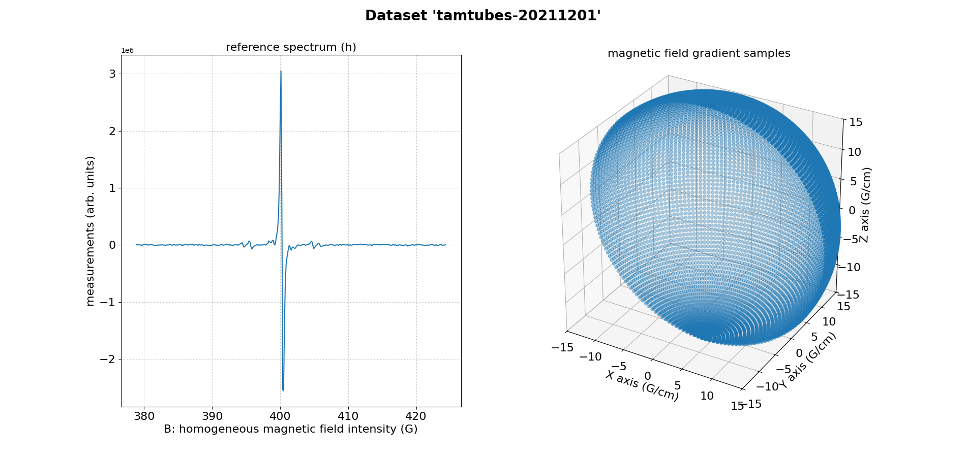
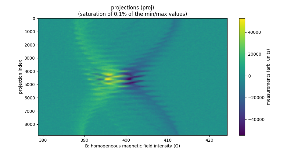
Sweep-width = 45.4733 G
Number of projections = 8836
Number of point per projection = 360
Field gradient magnitude = 20 G/cm

TAM and TEMPO (2D & 3D)

Solutions of TAM & TEMPO in two distinct tubes (2D)

The sample is made of two tubes. One containing 500 µL of a 2 mM TAM solution, the other one containing a 5 mM TEMPO solution. The tubes were placed in the cavity roughly a centimeter apart using a plastic holder.

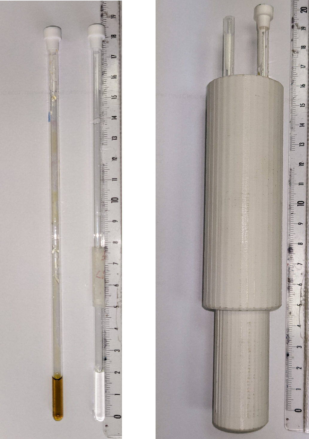
The dataset tam-and-tempo-tubes-2d-20210609 is two dimensional and has been acquired at LCBPT using an L-band Bruker spectrometer.

#--------------#
# Load dataset #
#--------------#
dtype = 'float32'
datasetname = 'tam-and-tempo-tubes-2d-20210609'
path_proj = datasets.get_path(datasetname + '-proj.pkl')
path_hmixt = datasets.get_path(datasetname + '-hmixt.pkl')
path_htam = datasets.get_path(datasetname + '-htam.pkl')
path_htempo = datasets.get_path(datasetname + '-htempo.pkl')
dataset_proj = io.load(path_proj, backend=backend, dtype=dtype) # load the dataset containing the projections
dataset_htam = io.load(path_htam, backend=backend, dtype=dtype) # load the dataset containing the reference spectrum of the TAM
dataset_htempo = io.load(path_htempo, backend=backend, dtype=dtype) # load the dataset containing the reference spectrum of the TEMPO
dataset_hmixt = io.load(path_hmixt, backend=backend, dtype=dtype) # load the dataset containing the reference spectrum of the whole sample (TAM + TEMPO)
B = dataset_proj['B'] # get B nodes from the loaded dataset
proj = dataset_proj['DAT'] # get projections data from the loaded dataset
fgrad = dataset_proj['FGRAD'] # get field gradient data from the loaded dataset
htam = dataset_htam['DAT'] # get TAM reference spectrum data from the loaded dataset
htempo = dataset_htempo['DAT'] # get TEMPO reference spectrum data from the loaded dataset
hmixt = dataset_htempo['DAT'] # get the TAM + TEMPO reference spectrum data from the loaded dataset (also equal to htam + htempo)

# ------------------------------------------------------------ #
# Compute and display several important acquisition parameters #
# ------------------------------------------------------------ #
print("Sweep-width = %g G" % (B[-1] - B[0]))
print("Number of projections = %d" % proj.shape[0])
print("Number of point per projection = %d" % proj.shape[1])
mu = backend.sqrt(fgrad[0]**2 + fgrad[1]**2) # magnitudes of the field gradient vectors (constant for this dataset)
print("Field gradient magnitude = %g G/cm" % mu[0])

#-----------------#
# Display dataset #
#-----------------#

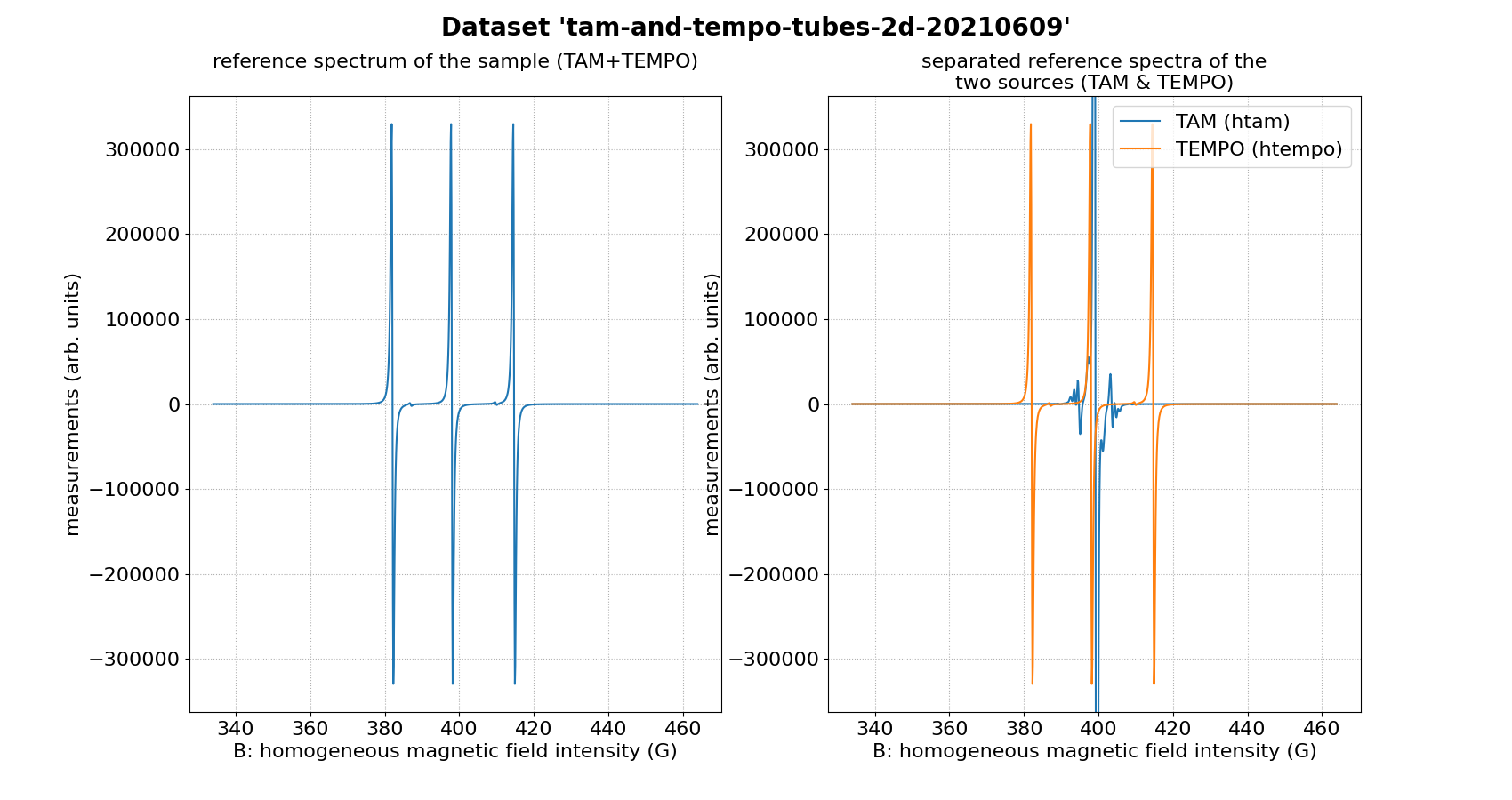
# display the reference spectrum of the whole sample (TAM + TEMPO)
plt.figure(figsize=(17, 9))
plt.subplot(1, 2, 1)
plt.plot(backend.to_numpy(B), backend.to_numpy(hmixt))
ax1 = plt.gca()
plt.grid(linestyle=':')
plt.xlabel('B: homogeneous magnetic field intensity (G)')
plt.ylabel('measurements (arb. units)')
plt.title('reference spectrum of the sample (TAM+TEMPO)\n')
for item in ([ax1.title, ax1.xaxis.label, ax1.yaxis.label] +
             ax1.get_xticklabels() + ax1.get_yticklabels()):
    item.set_fontsize(16)

# display the reference spectrum of the separated sources (TAM & TEMPO)
plt.subplot(1, 2, 2)
plt.plot(backend.to_numpy(B), backend.to_numpy(htam))
plt.plot(backend.to_numpy(B), backend.to_numpy(htempo))
ax2 = plt.gca()
ax2.set_ylim(ax1.get_ylim())
plt.grid(linestyle=':')
plt.xlabel('B: homogeneous magnetic field intensity (G)')
plt.ylabel('measurements (arb. units)')
plt.title('separated reference spectra of the\ntwo sources (TAM & TEMPO)')
plt.suptitle("Dataset '" + datasetname + "'",  weight='demibold', fontsize=20);
for item in ([ax2.title, ax2.xaxis.label, ax2.yaxis.label] +
             ax2.get_xticklabels() + ax2.get_yticklabels()):
    item.set_fontsize(16)
ax2.legend(['TAM (htam)', 'TEMPO (htempo)'], fontsize="16")

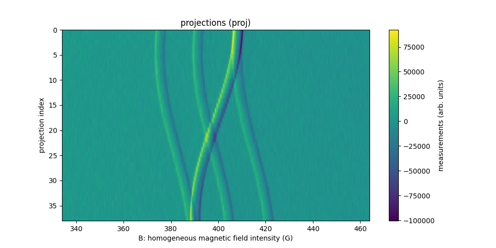
# display the projections
plt.figure(figsize=(10, 5))
extent = (B[0].item(), B[-1].item(), proj.shape[0] - 1, 0)
im_hdl = plt.imshow(backend.to_numpy(proj), extent=extent, aspect='auto')
cbar = plt.colorbar()
cbar.set_label('measurements (arb. units)')
plt.xlabel('B: homogeneous magnetic field intensity (G)')
plt.ylabel('projection index')
plt.title('projections (proj)')

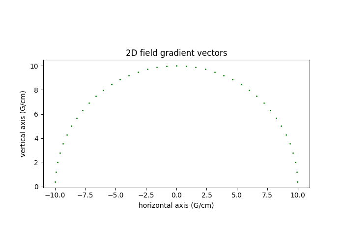
# display the field gradient vector associated to the measured projections
plt.figure(figsize=(7, 5))
plt.plot(backend.to_numpy(fgrad[0]), backend.to_numpy(fgrad[1]), 'go', markersize=1)
plt.gca().set_aspect('equal')
plt.xlabel("horizontal axis (G/cm)")
plt.ylabel("vertical axis (G/cm)")
_ = plt.title("2D field gradient vectors")

• 
• 
• 

Sweep-width = 129.892 G
Number of projections = 39
Number of point per projection = 1200
Field gradient magnitude = 10 G/cm

Solutions of TAM & TEMPO in two distinct tubes (3D)

The sample is the same as that presented in the previous section. The dataset tam-and-tempo-tubes-3d-20210609 is three dimensional and has been acquired at LCBPT using an L-band Bruker spectrometer.

#--------------#
# Load dataset #
#--------------#
dtype = 'float32'
datasetname = 'tam-and-tempo-tubes-3d-20210609'
path_proj = datasets.get_path(datasetname + '-proj.pkl')
path_htam = datasets.get_path(datasetname + '-htam.pkl')
path_htempo = datasets.get_path(datasetname + '-htempo.pkl')
dataset_proj = io.load(path_proj, backend=backend, dtype=dtype) # load the dataset containing the projections
dataset_htam = io.load(path_htam, backend=backend, dtype=dtype) # load the dataset containing the reference spectrum of the TAM
dataset_htempo = io.load(path_htempo, backend=backend, dtype=dtype) # load the dataset containing the reference spectrum of the TEMPO
B = dataset_proj['B'] # get B nodes from the loaded dataset
proj = dataset_proj['DAT'] # get projections data from the loaded dataset
fgrad = dataset_proj['FGRAD'] # get field gradient data from the loaded dataset
htam = dataset_htam['DAT'] # get TAM reference spectrum data from the loaded dataset
htempo = dataset_htempo['DAT'] # get TEMPO reference spectrum data from the loaded dataset

# ------------------------------------------------------------ #
# Compute and display several important acquisition parameters #
# ------------------------------------------------------------ #
print("Sweep-width = %g G" % (B[-1] - B[0]))
print("Number of projections = %d" % proj.shape[0])
print("Number of point per projection = %d" % proj.shape[1])
mu = backend.sqrt(fgrad[0]**2 + fgrad[1]**2 + fgrad[2]**2) # magnitudes of the field gradient vectors (constant for this dataset)
print("Field gradient magnitude = %g G/cm" % mu[0])

#-----------------#
# Display dataset #
#-----------------#

# display the reference spectrum of the first source (TAM)
plt.figure(figsize=(15, 5))
plt.subplot(1, 2, 1)
plt.plot(backend.to_numpy(B), backend.to_numpy(htam))
ax1 = plt.gca()
plt.grid(linestyle=':')
plt.xlabel('B: homogeneous magnetic field intensity (G)')
plt.ylabel('measurements (arb. units)')
plt.title('reference spectrum of the first source (TAM)')

# display the reference spectrum of the first source (TEMPO)
plt.subplot(1, 2, 2)
plt.plot(backend.to_numpy(B), backend.to_numpy(htempo))
ax2 = plt.gca()
ax2.set_ylim(ax1.get_ylim())
plt.grid(linestyle=':')
plt.xlabel('B: homogeneous magnetic field intensity (G)')
plt.ylabel('measurements (arb. units)')
plt.title('reference spectrum of the second source (TEMPO)')
plt.suptitle("Dataset '" + datasetname + "'",  weight='demibold');

# display the projections
plt.figure(figsize=(10, 5))
extent = (B[0].item(), B[-1].item(), proj.shape[0] - 1, 0)
im_hdl = plt.imshow(backend.to_numpy(proj), extent=extent, aspect='auto')
cbar = plt.colorbar()
cbar.set_label('measurements (arb. units)')
plt.xlabel('B: homogeneous magnetic field intensity (G)')
plt.ylabel('projection index')
_ = plt.title('projections (proj)')

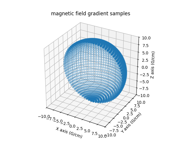
# display the field gradient vector associated to the measured projections
fig = plt.figure(figsize=(6, 5))
ax = fig.add_subplot(projection='3d')
ax.scatter(backend.to_numpy(fgrad[0]), backend.to_numpy(fgrad[1]), backend.to_numpy(fgrad[2]))
ax.set_xlim(-10, 10)
ax.set_ylim(-10, 10)
ax.set_zlim(-10, 10)
ax.set_aspect('equal', 'box')
ax.set_xlabel("X axis (G/cm)")
ax.set_ylabel("Y axis (G/cm)")
ax.set_zlabel("Z axis (G/cm)")
_ = plt.title('magnetic field gradient samples')

• 
• 
• 

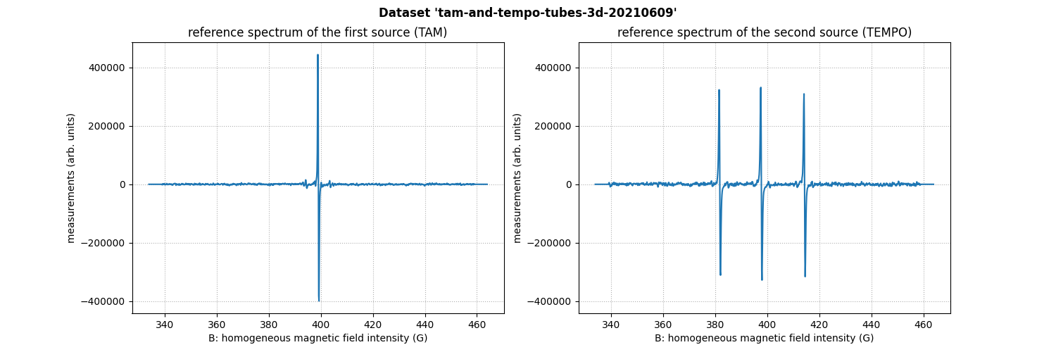
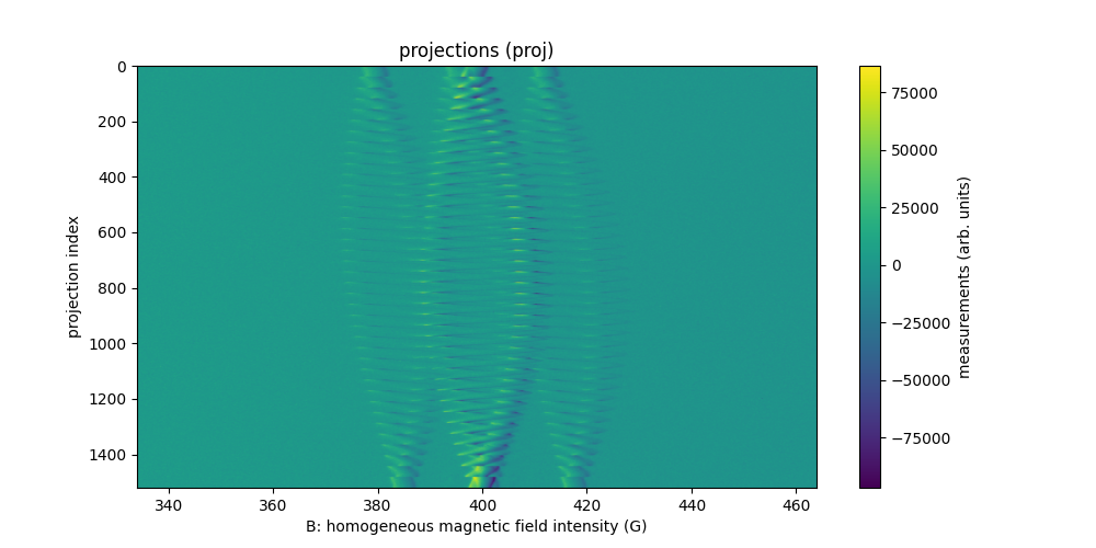
Sweep-width = 129.892 G
Number of projections = 1521
Number of point per projection = 1200
Field gradient magnitude = 10 G/cm

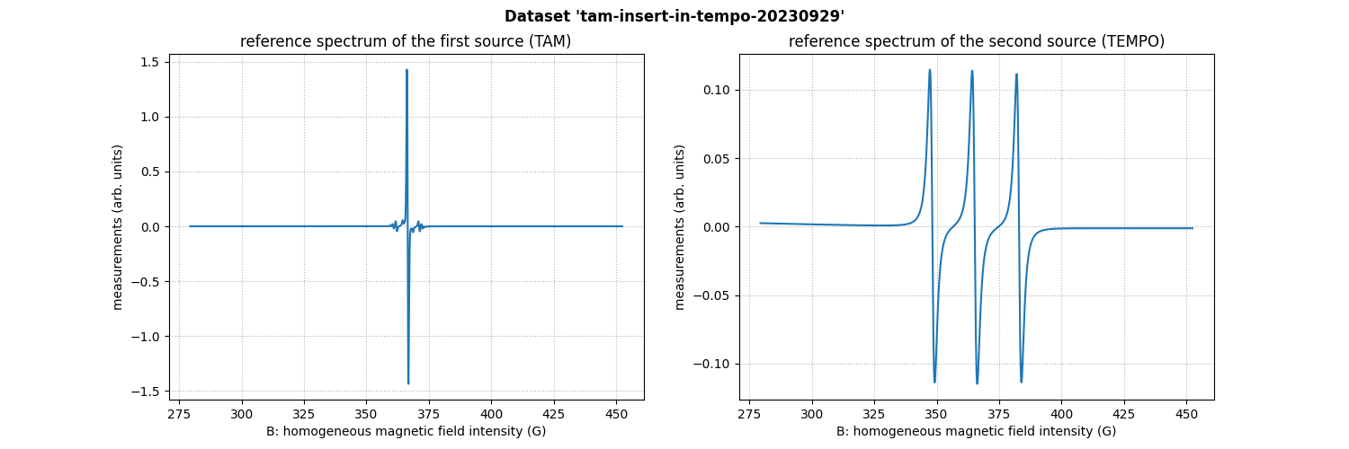
TAM solution insert into a TEMPO solution (3D)

The sample is made of a small eppendorf filled with a 12.5 mM solution of TAM placed inside a larger eppendorf filled with a 14 mM solution of TEMPO.

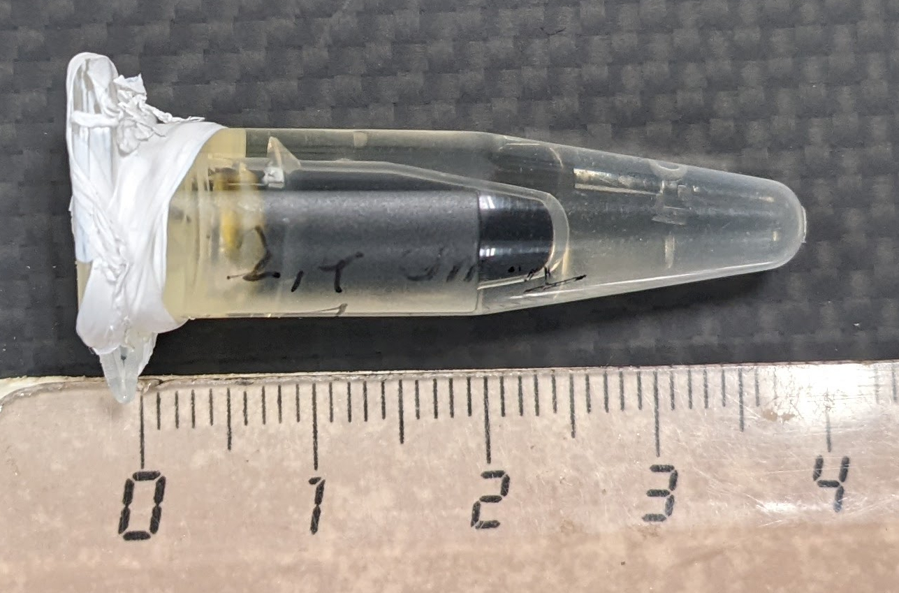
The dataset tam-insert-in-tempo-20230929 is three dimensional and was acquired at SFR ICAT University of Angers using an L-band Bruker spectrometer, with the kind help of Dr Raffaella Soleti.

#--------------#
# Load dataset #
#--------------#
dtype = 'float32'
datasetname = 'tam-insert-in-tempo-20230929'
path_proj = datasets.get_path(datasetname + '-proj.pkl')
path_htam = datasets.get_path(datasetname + '-htam.pkl')
path_htempo = datasets.get_path(datasetname + '-htempo.pkl')
dataset_proj = io.load(path_proj, backend=backend, dtype=dtype) # load the dataset containing the projections
dataset_htam = io.load(path_htam, backend=backend, dtype=dtype) # load the dataset containing the reference spectrum of the TAM
dataset_htempo = io.load(path_htempo, backend=backend, dtype=dtype) # load the dataset containing the reference spectrum of the TEMPO
B = dataset_proj['B'] # get B nodes from the loaded dataset
proj = dataset_proj['DAT'] # get projections data from the loaded dataset
fgrad = dataset_proj['FGRAD'] # get field gradient data from the loaded dataset
htam = dataset_htam['DAT'] # get TAM reference spectrum data from the loaded dataset
htempo = dataset_htempo['DAT'] # get TEMPO reference spectrum data from the loaded dataset

# ------------------------------------------------------------ #
# Compute and display several important acquisition parameters #
# ------------------------------------------------------------ #
print("Sweep-width = %g G" % (B[-1] - B[0]))
print("Number of projections = %d" % proj.shape[0])
print("Number of point per projection = %d" % proj.shape[1])
mu = backend.sqrt(fgrad[0]**2 + fgrad[1]**2 + fgrad[2]**2) # magnitudes of the field gradient vectors (constant for this dataset)
print("Field gradient magnitude = %g G/cm" % mu[0])

#-----------------#
# Display dataset #
#-----------------#

# display the reference spectrum of the first source (TAM)
plt.figure(figsize=(15, 5))
plt.subplot(1, 2, 1)
plt.plot(backend.to_numpy(B), backend.to_numpy(htam))
plt.grid(linestyle=':')
plt.xlabel('B: homogeneous magnetic field intensity (G)')
plt.ylabel('measurements (arb. units)')
plt.title('reference spectrum of the first source (TAM)')

# display the reference spectrum of the first source (TEMPO)
plt.subplot(1, 2, 2)
plt.plot(backend.to_numpy(B), backend.to_numpy(htempo))
plt.grid(linestyle=':')
plt.xlabel('B: homogeneous magnetic field intensity (G)')
plt.ylabel('measurements (arb. units)')
plt.title('reference spectrum of the second source (TEMPO)')
plt.suptitle("Dataset '" + datasetname + "'",  weight='demibold');

# display the projections
plt.figure(figsize=(10, 5))
extent = (B[0].item(), B[-1].item(), proj.shape[0] - 1, 0)
im_hdl = plt.imshow(backend.to_numpy(proj), extent=extent, aspect='auto')
cbar = plt.colorbar()
cbar.set_label('measurements (arb. units)')
plt.xlabel('B: homogeneous magnetic field intensity (G)')
plt.ylabel('projection index')
_ = plt.title('projections (proj)')

# display the field gradient vector associated to the measured projections
fig = plt.figure(figsize=(6, 5))
ax = fig.add_subplot(projection='3d')
ax.scatter(backend.to_numpy(fgrad[0]), backend.to_numpy(fgrad[1]), backend.to_numpy(fgrad[2]))
ax.set_xlim(-20, 20)
ax.set_ylim(-20, 20)
ax.set_zlim(-20, 20)
ax.set_aspect('equal', 'box')
ax.set_xlabel("X axis (G/cm)")
ax.set_ylabel("Y axis (G/cm)")
ax.set_zlabel("Z axis (G/cm)")
_ = plt.title('magnetic field gradient samples')

• 
• 
• 

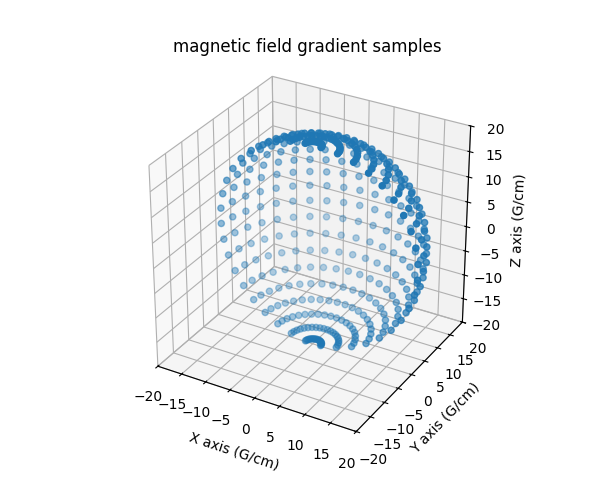
Sweep-width = 172.992 G
Number of projections = 400
Number of point per projection = 1600
Field gradient magnitude = 20 G/cm

Estimated memory usage: 363 MB