Note
Go to the end to download the full example code.
Fusillo soaked with 40H-TEMPO
3D image reconstruction of a ‘Fusillo’ (pasta with helical shape) soaked with an aqueous 4OH-TEMPO solution (see here for the sample and the dataset description).
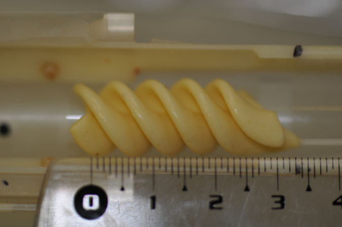
Picture of the sample.
Import needed modules
import numpy as np # for array manipulations
import matplotlib.pyplot as plt # tools for data visualization
import pyepri.backends as backends # to instanciate PyEPRI backends
import pyepri.datasets as datasets # to retrieve the path (on your own machine) of the demo dataset
import pyepri.displayers as displayers # tools for displaying images (with update along the computation)
import pyepri.processing as processing # tools for EPR image reconstruction
import pyepri.io as io # tools for loading EPR datasets (in BES3T or Python .PKL format)
Create backend
We create a numpy backend here because it should be available on your system (as a mandatory dependency of the PyEPRI package). You can try another backend (if available on your system) by uncommenting the appropriate line below (using a GPU backend may drastically reduce the computation time).
backend = backends.create_numpy_backend() # default numpy backend (CPU)
#backend = backends.create_torch_backend('cpu') # uncomment here for torch-cpu backend (CPU)
#backend = backends.create_cupy_backend() # uncomment here for cupy backend (GPU)
#backend = backends.create_torch_backend('cuda') # uncomment here for torch-gpu backend (GPU)
Load and display the input dataset
We load the fusillo-20091002 dataset (embedded with the PyEPRI
package) in float32 precision. Take a look to the comments for
changing the precision to float64 or replacing the embedded
dataset by one of your own dataset.
# ---------------------- #
# Load the input dataset #
# ---------------------- #
dtype = 'float32' # use 'float32' for single (32 bit) precision and 'float64' for double (64 bit) precision
path_proj = datasets.get_path('fusillo-20091002-proj.pkl') # or use your own dataset, e.g., path_proj = '~/my_projections.DSC'
path_h = datasets.get_path('fusillo-20091002-h.pkl') # or use your own dataset, e.g., path_h = '~/my_spectrum.DSC'
dataset_proj = io.load(path_proj, backend=backend, dtype=dtype) # load the dataset containing the projections
dataset_h = io.load(path_h, backend=backend, dtype=dtype) # load the dataset containing the reference spectrum
B = dataset_proj['B'] # get B nodes from the loaded dataset
proj = dataset_proj['DAT'] # get projections data from the loaded dataset
fgrad = dataset_proj['FGRAD'] # get field gradient data from the loaded dataset
h = dataset_h['DAT'] # get reference spectrum data from the loaded dataset

# -------------------------------------------------------- #
# Display the retrieved projections and reference spectrum #
# -------------------------------------------------------- #

# plot the reference spectrum
fig = plt.figure(figsize=(12, 5))
fig.add_subplot(1, 2, 1)
plt.plot(backend.to_numpy(B), backend.to_numpy(h))
plt.grid(linestyle=':')
plt.xlabel('B: homogeneous magnetic field intensity (G)')
plt.ylabel('measurements (arb. units)')
plt.title('reference spectrum (h)')

# plot the projections
fig.add_subplot(1, 2, 2)
extent = (B[0].item(), B[-1].item(), proj.shape[0] - 1, 0)
im_hdl = plt.imshow(backend.to_numpy(proj), extent=extent, aspect='auto')
cbar = plt.colorbar()
cbar.set_label('measurements (arb. units)')
plt.xlabel('B: homogeneous magnetic field intensity (G)')
plt.ylabel('projection index')
plt.title('projections (proj)')

# add suptitle and display the figure
plt.suptitle("Input dataset",  weight='demibold');
plt.show() # to keep the display persistent when the code is executed as a script
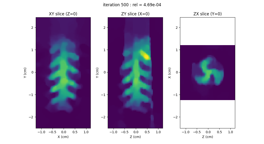
Configure and run the TV-regularized monosource image reconstruction
# ------------------------ #
# Set mandatory parameters #
# ------------------------ #
delta = .05; # sampling step in the same length unit as the provided field gradient coordinates (here cm)
out_shape = (100, 50, 50) # output image shape (number of pixels along each axes)
lbda = 500. # regularity parameter (arbitrary unit)

# ----------------------- #
# Set optional parameters #
# ----------------------- #
nitermax = 500 # maximal number of iterations
verbose = False # disable console verbose mode
video = True # enable video display
Ndisplay = 20 # refresh display rate (iteration per refresh)
eval_energy = False # disable TV-regularized least-square energy
                    # evaluation each Ndisplay iteration

# ------------------------------------------------------------------------ #
# Customize 3D image displayer (optional, used only when video=True above) #
# ------------------------------------------------------------------------ #
xgrid = (-(out_shape[1]//2) + np.arange(out_shape[1])) * delta # X-axis (horizontal) sampling grid
ygrid = (-(out_shape[0]//2) + np.arange(out_shape[0])) * delta # Y-axis (vertical) sampling grid
zgrid = (-(out_shape[2]//2) + np.arange(out_shape[2])) * delta # Z-axis (depth) sampling grid
grids = (ygrid, xgrid, zgrid) # spatial sampling grids
unit = 'cm' # provide length unit associated to the grids (used to label the image axes)
display_labels = True # display axes labels within subplots
adjust_dynamic = True # maximize displayed dynamic at each refresh
boundaries = 'same' # give all subplots the same axes boundaries (ensure same pixel size for
                    # each displayed slice)
displayFcn = lambda u : np.maximum(u, 0.) # threshold display (negative values are displayed as 0)
figsize=(11., 6.) # size (width and height in inches) of the displayed figure
displayer = displayers.create_3d_displayer(nsrc=1,
                                           figsize=figsize,
                                           displayFcn=displayFcn,
                                           units=unit,
                                           adjust_dynamic=adjust_dynamic,
                                           display_labels=display_labels,
                                           boundaries=boundaries,
                                           grids=grids)

# ---------------------------------------------------------- #
# Perform TV-regularized monosource EPR image reconstruction #
# ---------------------------------------------------------- #
out = processing.tv_monosrc(proj, B, fgrad, delta, h, lbda, out_shape,
                            backend=backend, init=None, tol=1e-4,
                            nitermax=nitermax,
                            eval_energy=eval_energy, verbose=verbose,
                            video=video, Ndisplay=Ndisplay,
                            displayer=displayer)
plt.show() # to keep the display persistent when the code is executed as a script
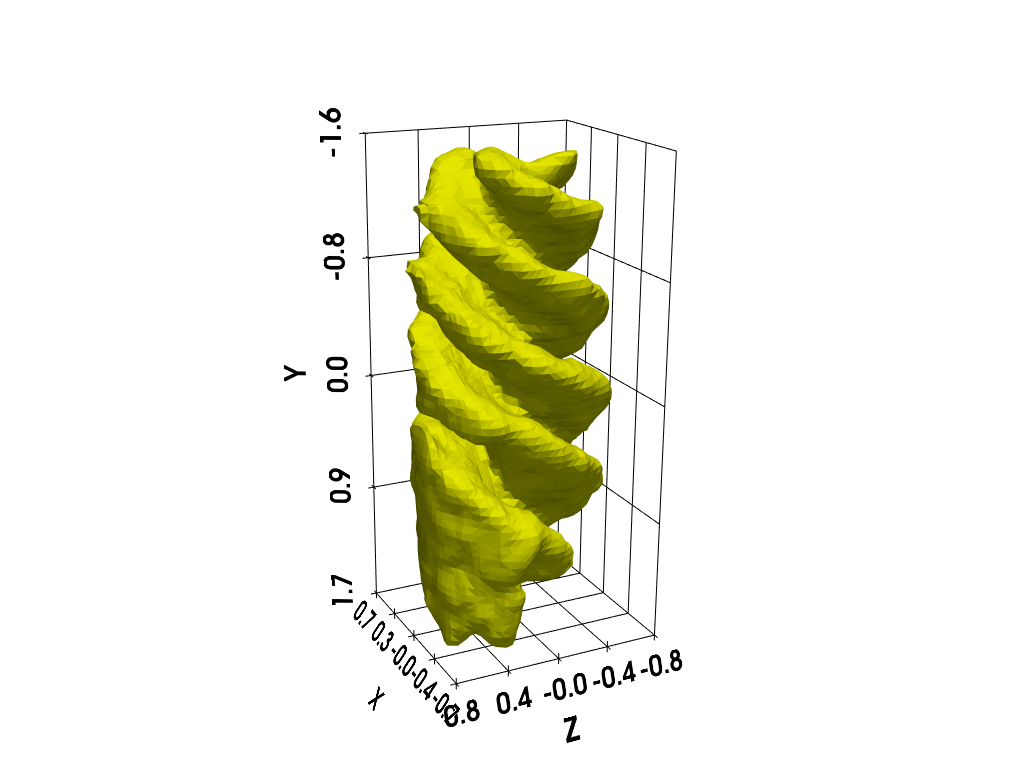
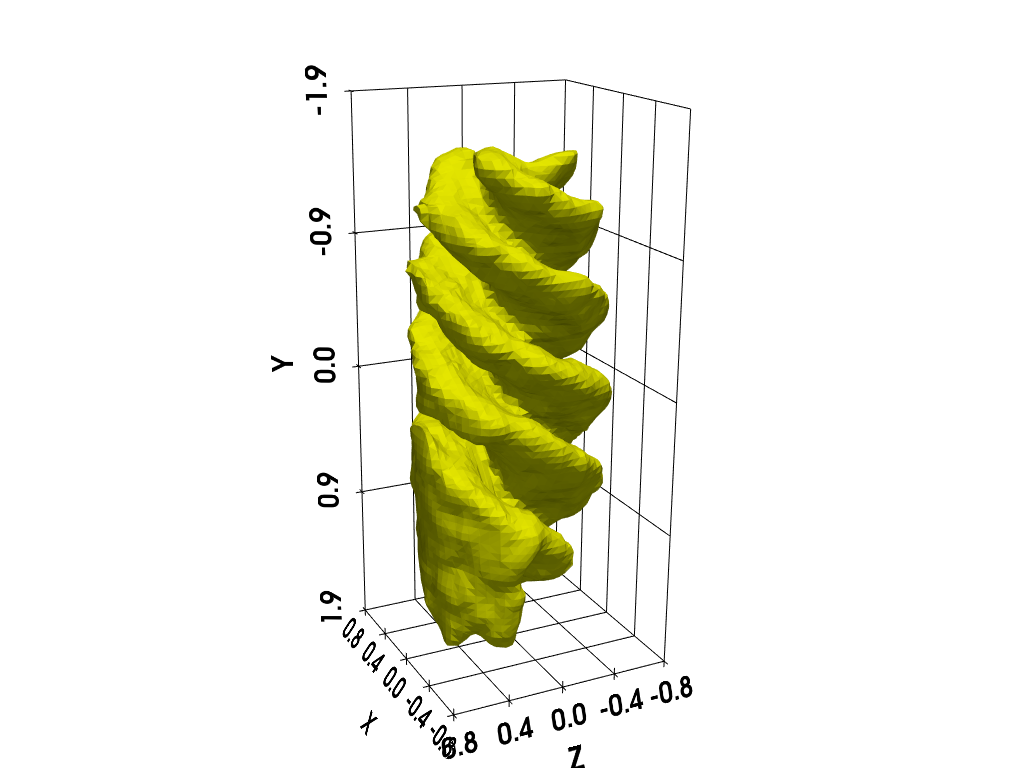
Isosurface rendering (requires working pyvista installation)
# additional import (pyvista)
import pyvista as pv # tools for rendering 3D volumes

# prepare isosurface display
x, y, z = np.meshgrid(xgrid, ygrid, zgrid, indexing='xy')
grid = pv.StructuredGrid(x, y, z)

# compute isosurface
vol = np.moveaxis(backend.to_numpy(out), (0,1,2), (2,1,0))
grid["vol"] = vol.flatten()
l1 = vol.max()
l0 = .2 * l1
isolevels = np.linspace(l0, l1, 10)
contours = grid.contour(isolevels)

# display isosurface
cpos = [(-8.2, -3.1, 4.1), (0.0, 0.0, 0.0), (0.3, -0.95, -0.14)]
p = pv.Plotter()
p.camera_position = cpos
labels = dict(ztitle='Z', xtitle='X', ytitle='Y')
p.add_mesh(contours, show_scalar_bar=False, color='#f7fe00')
p.show_grid(**labels, bounds=[-0.8, 0.8, -1.9, 1.9, -0.8, 0.8])
p.show()
Total running time of the script: (0 minutes 14.766 seconds)
Estimated memory usage: 413 MB