Note
Go to the end to download the full example code.
Tubes filled with TAM
3D image reconstruction of tubes filled with a solution of TAM (see here for the sample and the dataset description).
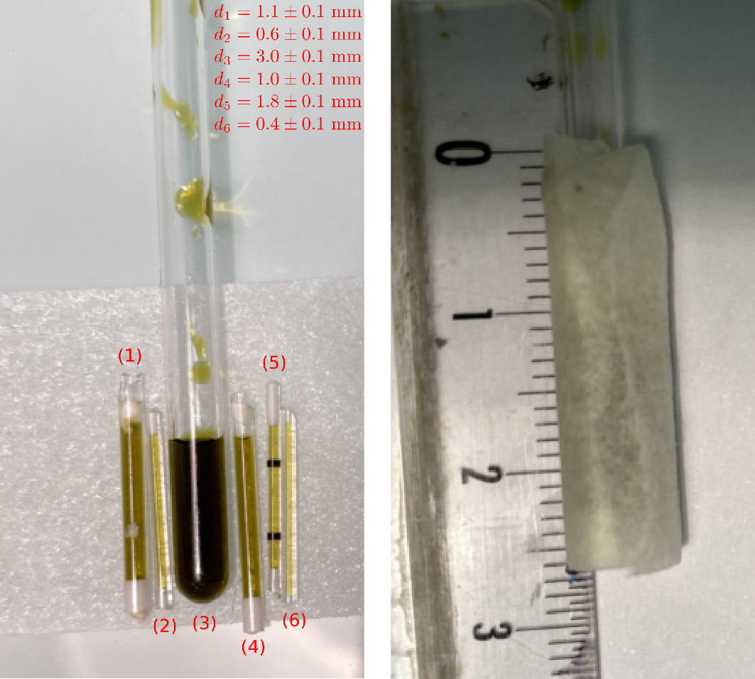
Picture of the sample.
Important: it should be noted that tubes (1) and (6) were badly sealed and leaked (partially for tube (1) and totally for tube (6)) during the experiment). This will affect the the upcoming image reconstructions.
Import needed modules
import numpy as np # for array manipulations
import matplotlib.pyplot as plt # tools for data visualization
import pyepri.backends as backends # to instanciate PyEPRI backends
import pyepri.datasets as datasets # to retrieve the path (on your own machine) of the demo dataset
import pyepri.displayers as displayers # tools for displaying images (with update along the computation)
import pyepri.processing as processing # tools for EPR image reconstruction
import pyepri.io as io # tools for loading EPR datasets (in BES3T or Python .PKL format)
Create backend
We create a numpy backend here because it should be available on your system (as a mandatory dependency of the PyEPRI package). You can try another backend (if available on your system) by uncommenting the appropriate line below (using a GPU backend may drastically reduce the computation time).
backend = backends.create_numpy_backend() # default numpy backend (CPU)
#backend = backends.create_torch_backend('cpu') # uncomment here for torch-cpu backend (CPU)
#backend = backends.create_cupy_backend() # uncomment here for cupy backend (GPU)
#backend = backends.create_torch_backend('cuda') # uncomment here for torch-gpu backend (GPU)
Load and display the input dataset
We load the tamtubes-20211201 dataset (embedded with the PyEPRI
package) in float32 precision. Take a look to the comments for
changing the precision to float64 or replacing the embedded
dataset by one of your own dataset.
# ---------------------- #
# Load the input dataset #
# ---------------------- #
dtype = 'float32' # use 'float32' for single (32 bit) precision and 'float64' for double (64 bit) precision
path_proj = datasets.get_path('tamtubes-20211201-proj.pkl') # or use your own dataset, e.g., path_proj = '~/my_projections.DSC'
path_h = datasets.get_path('tamtubes-20211201-h.pkl') # or use your own dataset, e.g., path_h = '~/my_spectrum.DSC'
dataset_proj = io.load(path_proj, backend=backend, dtype=dtype) # load the dataset containing the projections
dataset_h = io.load(path_h, backend=backend, dtype=dtype) # load the dataset containing the reference spectrum
B = dataset_proj['B'] # get B nodes from the loaded dataset
proj = dataset_proj['DAT'] # get projections data from the loaded dataset
fgrad = dataset_proj['FGRAD'] # get field gradient data from the loaded dataset
h = dataset_h['DAT'] # get reference spectrum data from the loaded dataset

# -------------------------------------------------------- #
# Display the retrieved projections and reference spectrum #
# -------------------------------------------------------- #

# plot the reference spectrum
fig = plt.figure(figsize=(12, 5))
fig.add_subplot(1, 2, 1)
plt.plot(backend.to_numpy(B), backend.to_numpy(h))
plt.grid(linestyle=':')
plt.xlabel('B: homogeneous magnetic field intensity (G)')
plt.ylabel('measurements (arb. units)')
plt.title('reference spectrum (h)')

# plot the projections
fig.add_subplot(1, 2, 2)
extent = (B[0].item(), B[-1].item(), proj.shape[0] - 1, 0)
im_hdl = plt.imshow(backend.to_numpy(proj), extent=extent, aspect='auto')
cbar = plt.colorbar()
cbar.set_label('measurements (arb. units)')
plt.xlabel('B: homogeneous magnetic field intensity (G)')
plt.ylabel('projection index')
plt.title('projections (proj)')

# add suptitle and display the figure
plt.suptitle("Input dataset",  weight='demibold');
plt.show() # to keep the display persistent when the code is executed as a script
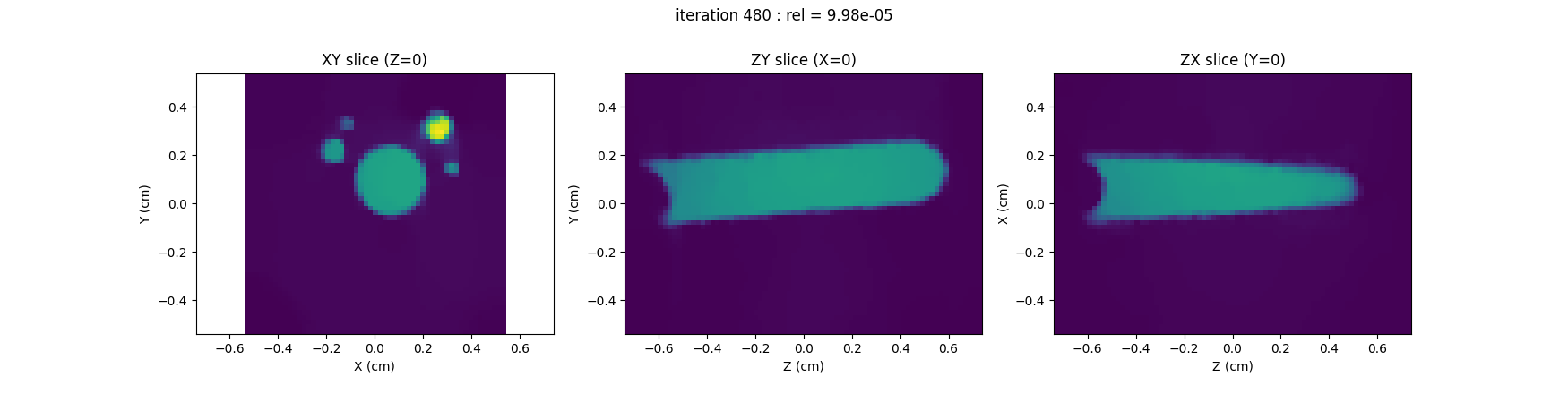
Configure and run the TV-regularized monosource image reconstruction
# ------------------------ #
# Set mandatory parameters #
# ------------------------ #
delta = .02; # sampling step in the same length unit as the provided field gradient coordinates (here cm)
out_shape = (55, 55, 75) # output image shape (number of pixels along each axes)
lbda = 5. # regularity parameter (arbitrary unit)

# ----------------------- #
# Set optional parameters #
# ----------------------- #
nitermax = 1000 # maximal number of iterations
verbose = False # disable console verbose mode
video = True # enable video display
Ndisplay = 20 # refresh display rate (iteration per refresh)
eval_energy = False # disable TV-regularized least-square energy
                    # evaluation each Ndisplay iteration

# ------------------------------------------------------------------------ #
# Customize 3D image displayer (optional, used only when video=True above) #
# ------------------------------------------------------------------------ #
xgrid = (-(out_shape[1]//2) + np.arange(out_shape[1])) * delta # X-axis (horizontal) sampling grid
ygrid = (-(out_shape[0]//2) + np.arange(out_shape[0])) * delta # Y-axis (vertical) sampling grid
zgrid = (-(out_shape[2]//2) + np.arange(out_shape[2])) * delta # Z-axis (depth) sampling grid
grids = (ygrid, xgrid, zgrid) # spatial sampling grids
unit = 'cm' # provide length unit associated to the grids (used to label the image axes)
display_labels = True # display axes labels within subplots
adjust_dynamic = True # maximize displayed dynamic at each refresh
boundaries = 'same' # give all subplots the same axes boundaries (ensure same pixel size for
                    # each displayed slice)
displayFcn = lambda u : np.maximum(u, 0.) # threshold display (negative values are displayed as 0)
figsize=(17.5, 4.5) # size (width and height in inches) of the displayed figure
displayer = displayers.create_3d_displayer(nsrc=1,figsize=figsize,
                                           displayFcn=displayFcn,
                                           units=unit,
                                           adjust_dynamic=adjust_dynamic,
                                           display_labels=display_labels,
                                           boundaries=boundaries,
                                           grids=grids)

# ---------------------------------------------------------- #
# Perform TV-regularized monosource EPR image reconstruction #
# ---------------------------------------------------------- #
out = processing.tv_monosrc(proj, B, fgrad, delta, h, lbda, out_shape,
                            backend=backend, init=None, tol=1e-4,
                            nitermax=nitermax,
                            eval_energy=eval_energy, verbose=verbose,
                            video=video, Ndisplay=Ndisplay,
                            displayer=displayer)
plt.show() # to keep the display persistent when the code is executed as a script
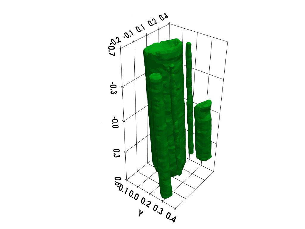
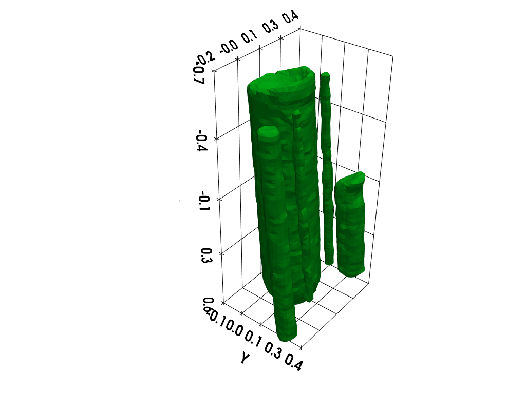
Isosurface rendering (requires working pyvista installation)
# additional import (pyvista)
import pyvista as pv # tools for rendering 3D volumes

# prepare isosurface display
x, y, z = np.meshgrid(xgrid, ygrid, zgrid, indexing='xy')
grid = pv.StructuredGrid(x, y, z)

# compute isosurface
vol = np.moveaxis(backend.to_numpy(out), (0,1,2), (2,1,0))
grid["vol"] = vol.flatten()
l1 = vol.max()
l0 = .2 * l1
isolevels = np.linspace(l0, l1, 10)
contours = grid.contour(isolevels)

# display isosurface
p = pv.Plotter()
cpos = [(-2.26, 1.84, -2.), (0, 0, 0), (0, 0, -1)]
p.camera_position = cpos
labels = dict(ztitle='Z', xtitle='X', ytitle='Y')
p.add_mesh(contours, show_scalar_bar=False, color='#01b517')
p.show_grid(**labels, bounds=[-0.2, 0.4, -0.1, 0.4, -0.7, 0.6])
p.show()
Total running time of the script: (0 minutes 10.410 seconds)
Estimated memory usage: 492 MB