Note
Go to the end to download the full example code.
Loading your own datasets in Python
How to load EPR datasets in Bruker BES3T (.DSC/.DTA), ASCII (.TXT), Matlab (.MAT), Numpy (.NPY) and Python Pickle (.PKL) format.
Dataset content and organization
To process your own data using PyEPRI, you need to load several signals (stored as arrays), typically:
A sequence of projections
proj: a two-dimensional array containing the measured projections (each row of this 2D array represents a single projection);The field gradient vector coordinates
fgrad: a two-dimensional array whose k-th column contains the coordinates of the field gradient vector associated with the k-th projection (i.e., the k-th row inproj);A reference spectrum
h: a one-dimensional array containing the reference (or zero-gradient) spectrum of your sample;The sampling grid
B: a one-dimensional array containing the values of the homogeneous magnetic field intensity used for sampling both the reference spectrumhand the measured projectionsproj(the reference spectrum and the projections are assumed to be sampled over the same grid).
Notes:
We do not impose any constraints on the choice of units. In our examples, we use centimeters (cm) for length units and gauss (G) for magnetic field units. Accordingly, field gradients are expressed in G/cm, and the sampling grid
Bis given in G. It is entirely possible to work with data expressed in other units (e.g., millimeters and millitesla). However, consistency is crucial: ifBis given in millitesla (mT) and the length unit is millimeter (mm), thenfgradmust be provided in mT/mm, and pixel sizes (used in image reconstruction experiments) must also be specified in millimeters.The dataset content depends on your specific application (e.g., no reference spectrum is needed of spectral-spatial imaging applications, on the contrary, the reference spectrum of each EPR source must be provided in case of source separation applications, …).
The PyEPRI package provides functions to easily load datasets stored in the Bruker BES3T format. However, datasets stored in other formats can also be used, as long as they are saved in a format that is easily readable by Python (e.g., .TXT, .PKL, .NPY, etc.).
In the next section, we will load (and display) a demonstration dataset embedded with PyEPRI package. In the following sections, we will illustrate how to adapt this code to load datasets in various formats.
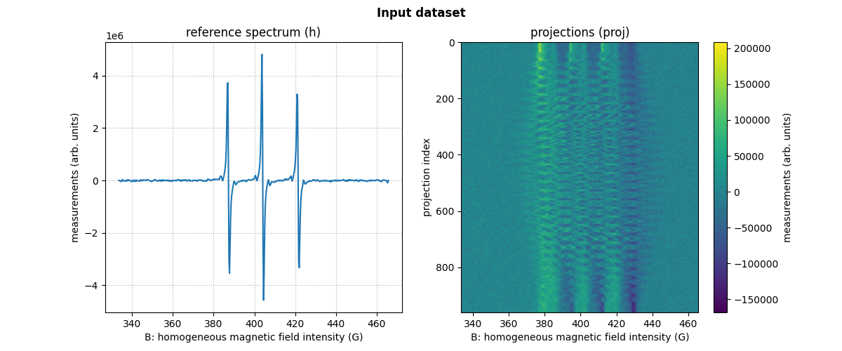
Loading a demonstration dataset
You should be able to load and display the demonstration
fusillo-20091002 dataset embedded with the PyEPRI package by
executing the following commands.
# --------------------- #
# Import needed modules #
# --------------------- #
import numpy as np # for numpy array manipulations
import scipy as sp # used here for .mat file loading
import matplotlib.pyplot as plt # to display signals
import pyepri.backends as backends # to instanciate PyEPRI backends
import pyepri.datasets as datasets # to retrieve the path (on your own machine) of the demo dataset
import pyepri.io as io # tools for loading EPR datasets (in BES3T or Python .PKL format)

# ---------------------------- #
# Create a numpy (CPU) backend #
# ---------------------------- #
backend = backends.create_numpy_backend()

# ----------------------------------------------------------------- #
# Load one demonstration dataset (fusillo pasta soaked with TEMPOL) #
# ----------------------------------------------------------------- #
dtype = 'float32' # use 'float32' for single (32 bit) precision and 'float64' for double (64 bit) precision
path_proj = datasets.get_path('fusillo-20091002-proj.pkl') # or use your own dataset, e.g., path_proj = '~/my_projections.DSC'
path_h = datasets.get_path('fusillo-20091002-h.pkl') # or use your own dataset, e.g., path_h = '~/my_spectrum.DSC'
dataset_proj = io.load(path_proj, backend=backend, dtype=dtype) # load the dataset containing the projections
dataset_h = io.load(path_h, backend=backend, dtype=dtype) # load the dataset containing the reference spectrum
B = dataset_proj['B'] # get B nodes from the loaded dataset
proj = dataset_proj['DAT'] # get projections data from the loaded dataset
fgrad = dataset_proj['FGRAD'] # get field gradient data from the loaded dataset
h = dataset_h['DAT'] # get reference spectrum data from the loaded dataset

# -------------------------------------------------------- #
# Display the retrieved projections and reference spectrum #
# -------------------------------------------------------- #

# plot the reference spectrum
fig = plt.figure(figsize=(12, 5))
fig.add_subplot(1, 2, 1)
plt.plot(backend.to_numpy(B), backend.to_numpy(h))
plt.grid(linestyle=':')
plt.xlabel('B: homogeneous magnetic field intensity (G)')
plt.ylabel('measurements (arb. units)')
plt.title('reference spectrum (h)')

# plot the projections
fig.add_subplot(1, 2, 2)
extent = (B[0].item(), B[-1].item(), proj.shape[0] - 1, 0)
im_hdl = plt.imshow(backend.to_numpy(proj), extent=extent, aspect='auto')
cbar = plt.colorbar()
cbar.set_label('measurements (arb. units)')
plt.xlabel('B: homogeneous magnetic field intensity (G)')
plt.ylabel('projection index')
plt.title('projections (proj)')

# add suptitle and display the figure
plt.suptitle("Input dataset",  weight='demibold');
plt.show()

# print the first four field gradient vector coordinates
print("Display of the first six field gradient vectors (one column = one vector)")
print("=========================================================================")
print(fgrad[:, :6])

Display of the first six field gradient vectors (one column = one vector)
=========================================================================
[[ 0.7081234   0.7008582   0.6864024   0.66490424  0.63658434  0.60173327]
 [ 0.03590915  0.10735904  0.17770746  0.24623263  0.3122315   0.375027  ]
 [13.982034   13.982034   13.982034   13.982034   13.982034   13.982034  ]]
Now, let us take a look at the path_proj and path_h
variables defined in the previous block. The paths displayed below
will be different on your own machine. They correspond to the
location where the example datasets are stored on your system (one
dataset containing the reference spectrum and another containing the
projections along with their associated field gradients).
print(path_proj)
print(path_h)
/home/remy/work/pyepri-github/datasets/fusillo-20091002-proj.pkl
/home/remy/work/pyepri-github/datasets/fusillo-20091002-h.pkl
Loading datasets stored in Bruker BES3T (.DSC/.DTA) format
Let us now assume that you have your own Bruker dataset organized in the same way — one dataset containing the reference spectrum and another containing the measured projections. You can manually provide the path to the location where the dataset is stored on your system.
In this example, we will use a dataset stored as follows (note that the paths will not be valid on your own system, as they correspond to where the files are stored on the machine used to generate this documentation):
reference spectrum: a set of two files (.DSC + .DTA) stored into
'/home/remy/work/pyepri-github/datasets/fusillo-20091002-h.DSC''/home/remy/work/pyepri-github/datasets/fusillo-20091002-h.DTA'
measured projections: a set of two files (.DSC + .DTA) stored into
'/home/remy/work/pyepri-github/datasets/fusillo-20091002-h.DSC''/home/remy/work/pyepri-github/datasets/fusillo-20091002-h.DTA'
You can use the PyEPRI function pyepri.io.load() to load each
dataset (provided that the .DSC and .DTA files of a given datasets
are both stored in the same directory). To that aim, simply provide
the absolute path to either the .DSC or the .DTA file of each
dataset (here we use the .DSC extension but we would get the same
result using the .DTA extension), as we do below.
Note: you must change below the path_h and path_proj
values to provide the paths where your Bruker files that are stored
on your system.
# Set path to the Bruker files (you must change the next two lines)
path_h = '/home/remy/work/pyepri-github/datasets/fusillo-20091002-h.DSC' # you must change the path here
path_proj = '/home/remy/work/pyepri-github/datasets/fusillo-20091002-proj.DSC'# you must change the path here

# Load the datasets (output are Python dict containing the data)
dataset_proj = io.load(path_proj, backend=backend, dtype=dtype) # load the dataset containing the projections
dataset_h = io.load(path_h, backend=backend, dtype=dtype) # load the dataset containing the reference spectrum

# extract the needed arrays from the loaded datasets
B = dataset_proj['B'] # get B nodes from the loaded dataset
proj = dataset_proj['DAT'] # get projections data from the loaded dataset
fgrad = dataset_proj['FGRAD'] # get field gradient data from the loaded dataset
h = dataset_h['DAT'] # get reference spectrum data from the loaded dataset
We can display the loaded reference spectrum and projections.
# plot the reference spectrum
fig = plt.figure(figsize=(12, 5))
fig.add_subplot(1, 2, 1)
plt.plot(backend.to_numpy(B), backend.to_numpy(h))
plt.grid(linestyle=':')
plt.xlabel('B: homogeneous magnetic field intensity (G)')
plt.ylabel('measurements (arb. units)')
plt.title('reference spectrum (h)')

# plot the projections
fig.add_subplot(1, 2, 2)
extent = (B[0].item(), B[-1].item(), proj.shape[0] - 1, 0)
im_hdl = plt.imshow(backend.to_numpy(proj), extent=extent, aspect='auto')
cbar = plt.colorbar()
cbar.set_label('measurements (arb. units)')
plt.xlabel('B: homogeneous magnetic field intensity (G)')
plt.ylabel('projection index')
plt.title('projections (proj)')

# add suptitle and display the figure
plt.suptitle("Input dataset",  weight='demibold');
plt.show()

# print the first four field gradient vector coordinates
print("Display of the first six field gradient vectors (one column = one vector)")
print("=========================================================================")
print(fgrad[:, :6])

Display of the first six field gradient vectors (one column = one vector)
=========================================================================
[[ 0.7081234   0.7008582   0.6864024   0.66490424  0.63658434  0.60173327]
 [ 0.03590915  0.10735904  0.17770746  0.24623263  0.3122315   0.375027  ]
 [13.982034   13.982034   13.982034   13.982034   13.982034   13.982034  ]]
Loading datasets stored in ASCII (.TXT) format
Whatever your EPR imaging system, you can probably manage to save your data in ASCII format (that is, a simple text file containing the numeric values of your measurements). You can for instance store one text file for each array to be retrieved using the following array-to-ascii conversion conventions:
One row of the array is stored as one row of the ASCII file;
The stored values are separated by a space character
' '.
In this example, we will work with files structured according to this convention, stored as follows:
A 1D array containing the reference spectrum stored at
/home/remy/work/pyepri-github/datasets/fusillo-20091002-h.txtA 2D array containing the projections (one row per projection) stored at
/home/remy/work/pyepri-github/datasets/fusillo-20091002-proj.txtA 2D array containing the field gradient vector coordinates (one column per projection) stored at
/home/remy/work/pyepri-github/datasets/fusillo-20091002-fgrad.txtA 1D array containing the sampling nodes stored at
/home/remy/work/pyepri-github/datasets/fusillo-20091002-B.txt
Such kind of ASCII data can be easily loaded using the the
loadtxt() function of the Numpy library, as we do below.
Note: you must change below the path_h, path_proj,
path_fgrad and path_B values to provide the paths where your
ASCII files are stored on your system.
# Set path to the ASCII files (you must change the next four lines)
path_h = '/home/remy/work/pyepri-github/datasets/fusillo-20091002-h.txt' # you must change the path here
path_proj = '/home/remy/work/pyepri-github/datasets/fusillo-20091002-proj.txt'# you must change the path here
path_fgrad = '/home/remy/work/pyepri-github/datasets/fusillo-20091002-fgrad.txt' # you must change the path here
path_B = '/home/remy/work/pyepri-github/datasets/fusillo-20091002-B.txt'# you must change the path here

# Load the data
B = backend.from_numpy(np.loadtxt(path_B, delimiter=' ', dtype=dtype))
proj = backend.from_numpy(np.loadtxt(path_proj, delimiter=' ', dtype=dtype))
fgrad = backend.from_numpy(np.loadtxt(path_fgrad, delimiter=' ', dtype=dtype))
h = backend.from_numpy(np.loadtxt(path_h, delimiter=' ', dtype=dtype))
Now we can display the loaded reference spectrum and projections
# plot the reference spectrum
fig = plt.figure(figsize=(12, 5))
fig.add_subplot(1, 2, 1)
plt.plot(backend.to_numpy(B), backend.to_numpy(h))
plt.grid(linestyle=':')
plt.xlabel('B: homogeneous magnetic field intensity (G)')
plt.ylabel('measurements (arb. units)')
plt.title('reference spectrum (h)')

# plot the projections
fig.add_subplot(1, 2, 2)
extent = (B[0].item(), B[-1].item(), proj.shape[0] - 1, 0)
im_hdl = plt.imshow(backend.to_numpy(proj), extent=extent, aspect='auto')
cbar = plt.colorbar()
cbar.set_label('measurements (arb. units)')
plt.xlabel('B: homogeneous magnetic field intensity (G)')
plt.ylabel('projection index')
plt.title('projections (proj)')

# add suptitle and display the figure
plt.suptitle("Input dataset",  weight='demibold');
plt.show()

# print the first four field gradient vector coordinates
print("Display of the first six field gradient vectors (one column = one vector)")
print("=========================================================================")
print(fgrad[:, :6])

Display of the first six field gradient vectors (one column = one vector)
=========================================================================
[[ 0.7081234   0.7008582   0.6864024   0.66490424  0.63658434  0.60173327]
 [ 0.03590915  0.10735904  0.17770745  0.24623263  0.3122315   0.375027  ]
 [13.982034   13.982034   13.982034   13.982034   13.982034   13.982034  ]]
Loading datasets stored in Matlab (.MAT) format
You can use Scipy’s loadmat function to load dataset stored in
Matlab (.MAT) format (this is particularly useful if you want, for
instance, apply some preprocessing to your data using EasySpin).
In this example, we will assume that the datasets were saved from
the Matlab console (using the Matlab’s save function). The .MAT
files contains the variables stored according the corresponding
variable names in the Matlab session. We will assume that those
Matlab variable names are those considered above (i.e., proj for
the measured projections, fgrad for the field gradient intensity
vectors, h for the reference spectrum and B for homogeneous
magnetic field sampling nodes), as well are there sizes (i.e., one
projection per row in proj, one field gradient vector per column
in fgrad).
We will consider a dataset made of two .MAT files:
/home/remy/work/pyepri-github/datasets/fusillo-20091002-h.mat: containing the h and B Matlab variables;/home/remy/work/pyepri-github/datasets/fusillo-20091002-proj.pkl: containing theproj,fgradandBvariables
This dataset has a bit of redudancy (since the variable B is
contained in both dataset) but this allows the two datasets to be
self consistent (in case one wants to load only one of them). You
can anyway adapt the code to change the dataset organization (this
demonstration example simply shows how to load .MAT content from
Python).
Note: you must change below the path_h and path_proj,
values to provide the paths where your .MAT files are stored on your
system.
# Set path to the .mat files (you must change the next two lines)
path_h = '/home/remy/work/pyepri-github/datasets/fusillo-20091002-h.mat' # you must change the path here
path_proj = '/home/remy/work/pyepri-github/datasets/fusillo-20091002-proj.mat'# you must change the path here

# Load the datasets (output are Python dict containing the data)
dataset_proj = sp.io.loadmat(path_proj) # load the dataset containing the projections
dataset_h = sp.io.loadmat(path_h) # load the dataset containing the reference spectrum

# extract the needed arrays from the loaded datasets
B = backend.from_numpy(dataset_proj['B'].astype(dtype).reshape(-1,)) # get B nodes from the loaded dataset
proj = backend.from_numpy(dataset_proj['proj'].astype(dtype)) # get projections data from the loaded dataset
fgrad = backend.from_numpy(dataset_proj['fgrad'].astype(dtype)) # get field gradient data from the loaded dataset
h = backend.from_numpy(dataset_h['h'].astype(dtype).reshape((-1,))) # get reference spectrum data from the loaded dataset
Now, let us display the loaded reference spectrum and projections.
# plot the reference spectrum
fig = plt.figure(figsize=(12, 5))
fig.add_subplot(1, 2, 1)
plt.plot(backend.to_numpy(B), backend.to_numpy(h))
plt.grid(linestyle=':')
plt.xlabel('B: homogeneous magnetic field intensity (G)')
plt.ylabel('measurements (arb. units)')
plt.title('reference spectrum (h)')

# plot the projections
fig.add_subplot(1, 2, 2)
extent = (B[0].item(), B[-1].item(), proj.shape[0] - 1, 0)
im_hdl = plt.imshow(backend.to_numpy(proj), extent=extent, aspect='auto')
cbar = plt.colorbar()
cbar.set_label('measurements (arb. units)')
plt.xlabel('B: homogeneous magnetic field intensity (G)')
plt.ylabel('projection index')
plt.title('projections (proj)')

# add suptitle and display the figure
plt.suptitle("Input dataset",  weight='demibold');
plt.show()

# print the first four field gradient vector coordinates
print("Display of the first six field gradient vectors (one column = one vector)")
print("=========================================================================")
print(fgrad[:, :6])

Display of the first six field gradient vectors (one column = one vector)
=========================================================================
[[ 0.7081234   0.7008582   0.6864024   0.66490424  0.63658434  0.60173327]
 [ 0.03590915  0.10735904  0.17770746  0.24623263  0.3122315   0.375027  ]
 [13.982034   13.982034   13.982034   13.982034   13.982034   13.982034  ]]
Loading datasets stored in Numpy (.NPY) format
Arrays can be easily saved in .npy format and later loaded using
NumPy’s save and load functions. In this example, we
consider such a dataset consisting of the following files:
A 1D array containing the reference spectrum stored at
/home/remy/work/pyepri-github/datasets/fusillo-20091002-h.npyA 2D array containing the projections (one row per projection) stored at
/home/remy/work/pyepri-github/datasets/fusillo-20091002-proj.npyA 2D array containing the field gradient vector coordinates (one column per projection) stored at
/home/remy/work/pyepri-github/datasets/fusillo-20091002-fgrad.npyA 1D array containing the sampling nodes stored at
/home/remy/work/pyepri-github/datasets/fusillo-20091002-B.npy
Note: you must change below the path_h, path_proj,
path_fgrad and path_B values to provide the paths where your
.NPY files are stored on your system.
# Set path to the ASCII files (you must change the next four lines)
path_h = '/home/remy/work/pyepri-github/datasets/fusillo-20091002-h.npy' # you must change the path here
path_proj = '/home/remy/work/pyepri-github/datasets/fusillo-20091002-proj.npy'# you must change the path here
path_fgrad = '/home/remy/work/pyepri-github/datasets/fusillo-20091002-fgrad.npy' # you must change the path here
path_B = '/home/remy/work/pyepri-github/datasets/fusillo-20091002-B.npy'# you must change the path here

# Load the data
B = backend.from_numpy(np.load(path_B).astype(dtype))
proj = backend.from_numpy(np.load(path_proj).astype(dtype))
fgrad = backend.from_numpy(np.load(path_fgrad).astype(dtype))
h = backend.from_numpy(np.load(path_h).astype(dtype))
We can display again the loaded reference spectrum and projections
# plot the reference spectrum
fig = plt.figure(figsize=(12, 5))
fig.add_subplot(1, 2, 1)
plt.plot(backend.to_numpy(B), backend.to_numpy(h))
plt.grid(linestyle=':')
plt.xlabel('B: homogeneous magnetic field intensity (G)')
plt.ylabel('measurements (arb. units)')
plt.title('reference spectrum (h)')

# plot the projections
fig.add_subplot(1, 2, 2)
extent = (B[0].item(), B[-1].item(), proj.shape[0] - 1, 0)
im_hdl = plt.imshow(backend.to_numpy(proj), extent=extent, aspect='auto')
cbar = plt.colorbar()
cbar.set_label('measurements (arb. units)')
plt.xlabel('B: homogeneous magnetic field intensity (G)')
plt.ylabel('projection index')
plt.title('projections (proj)')

# add suptitle and display the figure
plt.suptitle("Input dataset",  weight='demibold');
plt.show()

# print the first four field gradient vector coordinates
print("Display of the first six field gradient vectors (one column = one vector)")
print("=========================================================================")
print(fgrad[:, :6])

Display of the first six field gradient vectors (one column = one vector)
=========================================================================
[[ 0.7081234   0.7008582   0.6864024   0.66490424  0.63658434  0.60173327]
 [ 0.03590915  0.10735904  0.17770746  0.24623263  0.3122315   0.375027  ]
 [13.982034   13.982034   13.982034   13.982034   13.982034   13.982034  ]]
Loading datasets stored in Python pickle (.PKL) format
Python’s pickle module allows you to save dictionaries containing multiple arrays, making it possible to group all the data into a single file. In this example, we will consider a dataset made of two files:
/home/remy/work/pyepri-github/datasets/fusillo-20091002-h.pkl: a dictionnary with the following key-value content'DAT': the monodimensional array containing the measured values of the reference spectrum (that is, theharray);'B': the sampling magnetic field values associated to the reference spectrum.
/home/remy/work/pyepri-github/datasets/fusillo-20091002-proj.pkl: a dictionnary with the following key-value content'DAT': the two-dimensional array containing the measured projections (that is,projarray);'B': the sampling magnetic field values associated to the measured projections (should be the same as those contained in the reference spectrum file);'FGRAD': the two-dimensional array containing the field gradient vectors associated to the projections (that is, thefgradarray).
This is the format we chose to use for embedding the demonstration dataset in PyEPRI.
Note: you must change below the path_h and path_proj,
values to provide the paths where your .PKL files are stored on your
system.
# Set path to the .PKL files (you must change the next two lines)
path_h = '/home/remy/work/pyepri-github/datasets/fusillo-20091002-h.pkl' # you must change the path here
path_proj = '/home/remy/work/pyepri-github/datasets/fusillo-20091002-proj.pkl'# you must change the path here

# Load the datasets (output are Python dict containing the data)
dataset_proj = io.load(path_proj, backend=backend, dtype=dtype) # load the dataset containing the projections
dataset_h = io.load(path_h, backend=backend, dtype=dtype) # load the dataset containing the reference spectrum

# extract the needed arrays from the loaded datasets
B = dataset_proj['B'] # get B nodes from the loaded dataset
proj = dataset_proj['DAT'] # get projections data from the loaded dataset
fgrad = dataset_proj['FGRAD'] # get field gradient data from the loaded dataset
h = dataset_h['DAT'] # get reference spectrum data from the loaded dataset
We can display the loaded reference spectrum and projections.
# plot the reference spectrum
fig = plt.figure(figsize=(12, 5))
fig.add_subplot(1, 2, 1)
plt.plot(backend.to_numpy(B), backend.to_numpy(h))
plt.grid(linestyle=':')
plt.xlabel('B: homogeneous magnetic field intensity (G)')
plt.ylabel('measurements (arb. units)')
plt.title('reference spectrum (h)')

# plot the projections
fig.add_subplot(1, 2, 2)
extent = (B[0].item(), B[-1].item(), proj.shape[0] - 1, 0)
im_hdl = plt.imshow(backend.to_numpy(proj), extent=extent, aspect='auto')
cbar = plt.colorbar()
cbar.set_label('measurements (arb. units)')
plt.xlabel('B: homogeneous magnetic field intensity (G)')
plt.ylabel('projection index')
plt.title('projections (proj)')

# add suptitle and display the figure
plt.suptitle("Input dataset",  weight='demibold');
plt.show()

# print the first four field gradient vector coordinates
print("Display of the first six field gradient vectors (one column = one vector)")
print("=========================================================================")
print(fgrad[:, :6])
Display of the first six field gradient vectors (one column = one vector)
=========================================================================
[[ 0.7081234   0.7008582   0.6864024   0.66490424  0.63658434  0.60173327]
 [ 0.03590915  0.10735904  0.17770746  0.24623263  0.3122315   0.375027  ]
 [13.982034   13.982034   13.982034   13.982034   13.982034   13.982034  ]]
Total running time of the script: (0 minutes 3.403 seconds)
Estimated memory usage: 267 MB