Saving your results

Learn how to save your results in various data format.

After performing an image reconstruction operation, you’ll likely want to save your results. This tutorial shows how to do that in multiple formats. Let’s start by generating some data by rerunning the simplified 3D image reconstruction example on the fusillo sample dataset.

# --------------------- #
# Import needed modules #
# --------------------- #
import pyepri.apodization as apodization # tools for creating apodization profiles
import pyepri.backends as backends # to instanciate PyEPRI backends
import pyepri.datasets as datasets # to retrieve the path (on your own machine) of the demo dataset
import pyepri.displayers as displayers # tools for displaying images (with update along the computation)
import pyepri.monosrc as monosrc # tools related to standard EPR operators (projection, backprojection, ...)
import pyepri.multisrc as multisrc # tools related to multisources EPR operators (projection, backprojection, ...)
import pyepri.spectralspatial as ss # tools related to spectral spatial EPR operators (projection, backprojection, ...)
import pyepri.processing as processing # tools for EPR image reconstruction
import pyepri.io as io # tools for loading EPR datasets (in BES3T or Python .PKL format)

# ---------------------------- #
# Create a numpy (CPU) backend #
# ---------------------------- #
backend = backends.create_numpy_backend()

# ----------------------------------------------------------------- #
# Load one demonstration dataset (fusillo pasta soaked with TEMPOL) #
# ----------------------------------------------------------------- #
dtype = 'float32' # use 'float32' for single (32 bit) precision and 'float64' for double (64 bit) precision
path_proj = datasets.get_path('fusillo-20091002-proj.pkl') # or use your own dataset, e.g., path_proj = '~/my_projections.DSC'
path_h = datasets.get_path('fusillo-20091002-h.pkl') # or use your own dataset, e.g., path_h = '~/my_spectrum.DSC'
dataset_proj = io.load(path_proj, backend=backend, dtype=dtype) # load the dataset containing the projections
dataset_h = io.load(path_h, backend=backend, dtype=dtype) # load the dataset containing the reference spectrum
B = dataset_proj['B'] # get B nodes from the loaded dataset
proj = dataset_proj['DAT'] # get projections data from the loaded dataset
fgrad = dataset_proj['FGRAD'] # get field gradient data from the loaded dataset
h = dataset_h['DAT'] # get reference spectrum data from the loaded dataset

# ----------------------------------------------------- #
# Configure and run TV-regularized image reconstruction #
# ----------------------------------------------------- #
delta = .1; # sampling step in the same length unit as the provided field gradient coordinates (here cm)
out_shape = (50, 25, 25) # output image shape (number of pixels along each axis)
lbda = 500. # regularity parameter (arbitrary unit)
displayer = displayers.create_3d_displayer(nsrc=1, figsize=(11., 6.), display_labels=True)
out = processing.tv_monosrc(proj, B, fgrad, delta, h, lbda, out_shape, backend=backend,
                            init=None, tol=1e-4, nitermax=500, eval_energy=False,
                            verbose=False, video=True, Ndisplay=20, displayer=displayer)

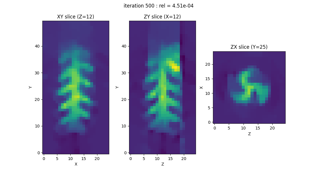
This script calculated an array out containing the values of the reconstructed image. To make the saving process a bit more complex, we show below how to save out together with the dataset variables (proj, h, B, and fgrad) and the reconstruction parameters (delta, lbda). You can adapt the code by removing or adding arrays as needed.

Exporting results in Python Pickel (.PKL) format

Exporting in Python Pickle format (.pkl) is the most suitable method if you want to save your results for later use in Python. It is recommended to convert the arrays into Numpy arrays (in case your backend is not a Numpy one), as we do below.

Note: make sure to change the value of the path variable below to specify a valid location and filenane for the final exported file.

# --------------------- #
# Import needed modules #
# --------------------- #
import pickle

# --------------------------------------------------- #
# Gather data to be exported into a Python dictionary #
# --------------------------------------------------- #
data = {'out': backend.to_numpy(out), # reconstructed EPR image (converted into a Numpy array)
        'proj': backend.to_numpy(proj), # projections (converted into a Numpy array)
        'fgrad': backend.to_numpy(fgrad), # field gradient vectors (converted into a Numpy array)
        'h': backend.to_numpy(h), # reference spectrum (converted into a Numpy array)
        'B': backend.to_numpy(h), # sampling nodes (converted into a Numpy array)
        'delta': delta, # spatial sampling step (pixel size) for the reconstructed image (out)
        'lbda': lbda, # regularity parameter (TV weight) used in the reconstruction process
        }

# --------------------------------------- #
# Saving the data in Python Pickle format #
# --------------------------------------- #
path = '/tmp/exported_data.pkl' # change here to specify the desired location and filename for the final exported file
with open(path, 'wb') as f:
    pickle.dump(data, f)

To load the exported data in a new Python session, you can do the following.

# ---------------------------------------- #
# Reload the data into a Python dictionary #
# ---------------------------------------- #
path = '/tmp/exported_data.pkl' # path towards your exported .pkl file
with open(path, 'rb') as f:
    data = pickle.load(f)

# ------------------------------------------------------------------ #
# Extract the data (convert the Numpy arrays to the appropriate type #
# depending on your backend)                                         #
# ------------------------------------------------------------------ #

# retrieve arrays (perform backend conversion)
out = backend.from_numpy(data['out']) # reconstructed EPR image
proj = backend.from_numpy(data['proj']) # projections
fgrad = backend.from_numpy(data['fgrad']) # field gradient vectors
h = backend.from_numpy(data['h']) # reference spectrum
B = backend.from_numpy(data['B']) # sampling nodes

# retrieve floats (no need of conversion here)
delta = data['delta'] # spatial sampling step (pixel size) for the reconstructed image (out)
lbda = data['lbda'] # regularity parameter (TV weight) used in the reconstruction process

Exporting results in Matlab (.MAT) format

Saving in the .MAT format is done similarly using the savemat function from SciPy.

# --------------------- #
# Import needed modules #
# --------------------- #
import scipy

# --------------------------------------------------- #
# Gather data to be exported into a Python dictionary #
# --------------------------------------------------- #
data = {'out': backend.to_numpy(out), # reconstructed EPR image (converted into a Numpy array)
        'proj': backend.to_numpy(proj), # projections (converted into a Numpy array)
        'fgrad': backend.to_numpy(fgrad), # field gradient vectors (converted into a Numpy array)
        'h': backend.to_numpy(h), # reference spectrum (converted into a Numpy array)
        'B': backend.to_numpy(h), # sampling nodes (converted into a Numpy array)
        'delta': delta, # spatial sampling step (pixel size) for the reconstructed image (out)
        'lbda': lbda, # regularity parameter (TV weight) used in the reconstruction process
        }

# --------------------------------------- #
# Saving the data in Python Pickle format #
# --------------------------------------- #
path = '/tmp/exported_data.mat' # change here to specify the desired location and filename for the final exported file
scipy.io.savemat(path, data)

The exported dataset can be loaded from a Matlab console using Matlab’s function load. If you need to load again the data in Python, however, since Matlab process all variables as matrices, you will need to reshape 1D arrays and scalar numbers after loading them from the .mat file, as we do below.

# ---------------------------------------- #
# Reload the data into a Python dictionary #
# ---------------------------------------- #
path = '/tmp/exported_data.mat' # path towards your exported .mat file
data = scipy.io.loadmat(path)

# ------------------------------------------------------------------ #
# Extract the data (convert the Numpy arrays to the appropriate type #
# depending on your backend)                                         #
# ------------------------------------------------------------------ #

# retrieve arrays (perform backend conversion)
out = backend.from_numpy(data['out']) # reconstructed EPR image
proj = backend.from_numpy(data['proj']) # projections
fgrad = backend.from_numpy(data['fgrad']) # field gradient vectors
h = backend.from_numpy(data['h']).reshape((-1,)) # reference spectrum (reshaped as a 1D array)
B = backend.from_numpy(data['B'].reshape((-1,))) # sampling nodes (reshaped as a 1D array)

# retrieve floats (those values are stored as 2D arrays containing a
# single element, we use .item() to extract the scalar value they contain
delta = data['delta'].item() # spatial sampling step (pixel size) for the reconstructed image (out)
lbda = data['lbda'].item() # regularity parameter (TV weight) used in the reconstruction process

Exporting results in ASCII (.TXT) format

Saving in ASCII format is also useful, as it is universal and easy to use. However, it requires saving each variable to a separate file, as shown below.

Note: We use the NumPy function savetxt to export arrays in ASCII format (which requires converting them to NumPy arrays). In this process, scalar variables must be converted into arrays. Also, 3D arrays must be reshaped into 2D arrays. To make the saving/loading process more automatic, we also save the 3D array shape in ASCII format.

# --------------------- #
# Import needed modules #
# --------------------- #
import numpy as np

# --------------------------------------------------- #
# Export data in ASCII format (one file per variable) #
# --------------------------------------------------- #

# set path (change here to specify the desired location and filename
# for the final exported file)
path_out_shape = "/tmp/out_shape.txt"
path_out = "/tmp/out.txt"
path_proj = "/tmp/proj.txt"
path_h = "/tmp/h.txt"
path_B = "/tmp/B.txt"
path_delta = "/tmp/delta.txt"
path_lbda = "/tmp/lbda.txt"

# save variables in ASCII format (including 3D -> 2D and scalar ->
# array conversion)
np.savetxt(path_out_shape, out.shape, delimiter=' ') # reshape 3D -> 2D done here
np.savetxt(path_out, backend.to_numpy(out.reshape(out.shape[0], out.shape[1] * out.shape[2])), delimiter=' ') # reshape 3D -> 2D done here
np.savetxt(path_proj, backend.to_numpy(proj), delimiter=' ')
np.savetxt(path_h, backend.to_numpy(h), delimiter=' ')
np.savetxt(path_B, backend.to_numpy(B), delimiter=' ')
np.savetxt(path_delta, np.array([delta]), delimiter=' ') # scalar -> array conversion done here
np.savetxt(path_lbda, np.array([lbda]), delimiter=' ') # scalar -> array conversion done here

To load again the data in a Python session, you can use the following.

# set path (change here to the paths towards your exported files)
path_out_shape = "/tmp/out_shape.txt"
path_out = "/tmp/out.txt"
path_proj = "/tmp/proj.txt"
path_h = "/tmp/h.txt"
path_B = "/tmp/B.txt"
path_delta = "/tmp/delta.txt"
path_lbda = "/tmp/lbda.txt"

# loading data (including 2D -> 3D and array -> scalar conversions)
out_shape = tuple(int(s.item()) for s in np.loadtxt(path_out_shape, delimiter=' ')) # retrieve 3D output shape
out = np.loadtxt(path_out, delimiter=' ').reshape(out_shape) # reshape 2D -> 3D done here
proj = np.loadtxt(path_proj, delimiter=' ')
h = np.loadtxt(path_h, delimiter=' ')
B = np.loadtxt(path_B, delimiter=' ')
delta = np.loadtxt(path_delta, delimiter=' ').item() # array -> scalar conversion done here
lbda = np.loadtxt(path_lbda, delimiter=' ').item() # array -> scalar conversion done here

Estimated memory usage: 251 MB