Check your PyEPRI installation and try EPR image reconstruction

Check that PyEPRI is correctly installed and run your first EPR image reconstruction experiment using PyEPRI.

Before following this tutorial, make sure you have installed PyEPRI on your machine (see the Installation section).

Loading PyEPRI modules

With PyEPRI correctly installed on your machine, you should be able to execute the following module import commands into a Python console (make sure you have activated the virtual environment in which PyEPRI was installed).

import pyepri.apodization as apodization # tools for creating apodization profiles
import pyepri.backends as backends # to instanciate PyEPRI backends
import pyepri.datasets as datasets # to retrieve the path (on your own machine) of the demo dataset
import pyepri.displayers as displayers # tools for displaying images (with update along the computation)
import pyepri.monosrc as monosrc # tools related to standard EPR operators (projection, backprojection, ...)
import pyepri.multisrc as multisrc # tools related to multisources EPR operators (projection, backprojection, ...)
import pyepri.spectralspatial as ss # tools related to spectral spatial EPR operators (projection, backprojection, ...)
import pyepri.processing as processing # tools for EPR image reconstruction
import pyepri.io as io # tools for loading EPR datasets (in BES3T or Python .PKL format)

If those modules import do not raise any error, PyEPRI is likely correctly installed on your system. You should be able to use it and reproduce all experiments provided in the tutorials and adapt them to process your own data.

Simplified EPR image reconstruction experiment

We will now test a simplified 3D RPE image reconstruction experiment. The commands below correspond to a concise and highly simplified version of a more detailed tutorial (see the full version here) which includes more advanced display configuration as well as 3D visualization of the reconstructed image.

# ---------------------------- #
# Create a numpy (CPU) backend #
# ---------------------------- #
backend = backends.create_numpy_backend()

# ----------------------------------------------------------------- #
# Load one demonstration dataset (fusillo pasta soaked with TEMPOL) #
# ----------------------------------------------------------------- #
dtype = 'float32' # use 'float32' for single (32 bit) precision and 'float64' for double (64 bit) precision
path_proj = datasets.get_path('fusillo-20091002-proj.pkl') # or use your own dataset, e.g., path_proj = '~/my_projections.DSC'
path_h = datasets.get_path('fusillo-20091002-h.pkl') # or use your own dataset, e.g., path_h = '~/my_spectrum.DSC'
dataset_proj = io.load(path_proj, backend=backend, dtype=dtype) # load the dataset containing the projections
dataset_h = io.load(path_h, backend=backend, dtype=dtype) # load the dataset containing the reference spectrum
B = dataset_proj['B'] # get B nodes from the loaded dataset
proj = dataset_proj['DAT'] # get projections data from the loaded dataset
fgrad = dataset_proj['FGRAD'] # get field gradient data from the loaded dataset
h = dataset_h['DAT'] # get reference spectrum data from the loaded dataset

# ----------------------------------------------------- #
# Configure and run TV-regularized image reconstruction #
# ----------------------------------------------------- #
delta = .1; # sampling step in the same length unit as the provided field gradient coordinates (here cm)
out_shape = (50, 25, 25) # output image shape (number of pixels along each axis)
lbda = 500. # regularity parameter (arbitrary unit)
displayer = displayers.create_3d_displayer(nsrc=1, figsize=(11., 6.), display_labels=True)
out = processing.tv_monosrc(proj, B, fgrad, delta, h, lbda, out_shape, backend=backend,
                            init=None, tol=1e-4, nitermax=500, eval_energy=False,
                            verbose=False, video=True, Ndisplay=20, displayer=displayer)

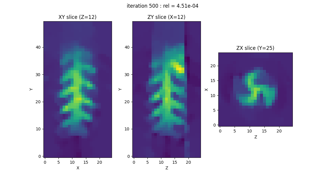
By executing the above commands on your machine, you should be able to visualize the evolution of the image (specifically, three slices of the image) throughout the iterations of the reconstruction algorithm. The image displayed above corresponds to the result obtained at the end of the iterative process—either when it has converged or when the maximum number of iterations specified by the user has been reached.

If you were able to successfully run all the commands presented here, then everything is set up to reproduce the experiments featured in the tutorials throughout this documentation. You can skip the following Troubleshooting section and proceed confidently to the next tutorial.

Troubleshooting

• Make sure that you have a working installation of Python on your system (you should be able to execute basic Python commands, through a Python console or an Integrated Development Environment).

• Make sure that you complete the installation of PyEPRI (see the Installation section).

• Make sure that the virtual environment in which PyEPRI was installed is activated when running the Python commands shown here. You can refer to the video tutorials in the Installation section for guidance on how to activate it.

• If you still encounter difficulties, feel free to ask for help here or to open a bug issue (if you feel that there is something wrong with the package itself).

Estimated memory usage: 239 MB