Interactive tools for image visualization

Learn about 3D and 4D image visualization tools from PyEPRI (require PyEPRI >= 1.1.1).

Interactive 3D image viewers

Let’s start by generating some data by rerunning the simplified 3D image reconstruction example on the fusillo sample dataset.

# --------------------- #
# Import needed modules #
# --------------------- #
import pyepri.apodization as apodization # tools for creating apodization profiles
import pyepri.backends as backends # to instanciate PyEPRI backends
import pyepri.datasets as datasets # to retrieve the path (on your own machine) of the demo dataset
import pyepri.displayers as displayers # tools for displaying images (with update along the computation)
import pyepri.monosrc as monosrc # tools related to standard EPR operators (projection, backprojection, ...)
import pyepri.multisrc as multisrc # tools related to multisources EPR operators (projection, backprojection, ...)
import pyepri.spectralspatial as ss # tools related to spectral spatial EPR operators (projection, backprojection, ...)
import pyepri.processing as processing # tools for EPR image reconstruction
import pyepri.io as io # tools for loading EPR datasets (in BES3T or Python .PKL format)

# ---------------------------- #
# Create a numpy (CPU) backend #
# ---------------------------- #
backend = backends.create_numpy_backend()

# ----------------------------------------------------------------- #
# Load one demonstration dataset (fusillo pasta soaked with TEMPOL) #
# ----------------------------------------------------------------- #
dtype = 'float32' # use 'float32' for single (32 bit) precision and 'float64' for double (64 bit) precision
path_proj = datasets.get_path('fusillo-20091002-proj.pkl') # or use your own dataset, e.g., path_proj = '~/my_projections.DSC'
path_h = datasets.get_path('fusillo-20091002-h.pkl') # or use your own dataset, e.g., path_h = '~/my_spectrum.DSC'
dataset_proj = io.load(path_proj, backend=backend, dtype=dtype) # load the dataset containing the projections
dataset_h = io.load(path_h, backend=backend, dtype=dtype) # load the dataset containing the reference spectrum
B = dataset_proj['B'] # get B nodes from the loaded dataset
proj = dataset_proj['DAT'] # get projections data from the loaded dataset
fgrad = dataset_proj['FGRAD'] # get field gradient data from the loaded dataset
h = dataset_h['DAT'] # get reference spectrum data from the loaded dataset

# ----------------------------------------------------- #
# Configure and run TV-regularized image reconstruction #
# ----------------------------------------------------- #
delta = .1; # sampling step in the same length unit as the provided field gradient coordinates (here cm)
out_shape = (50, 25, 25) # output image shape (number of pixels along each axis)
lbda = 500. # regularity parameter (arbitrary unit)
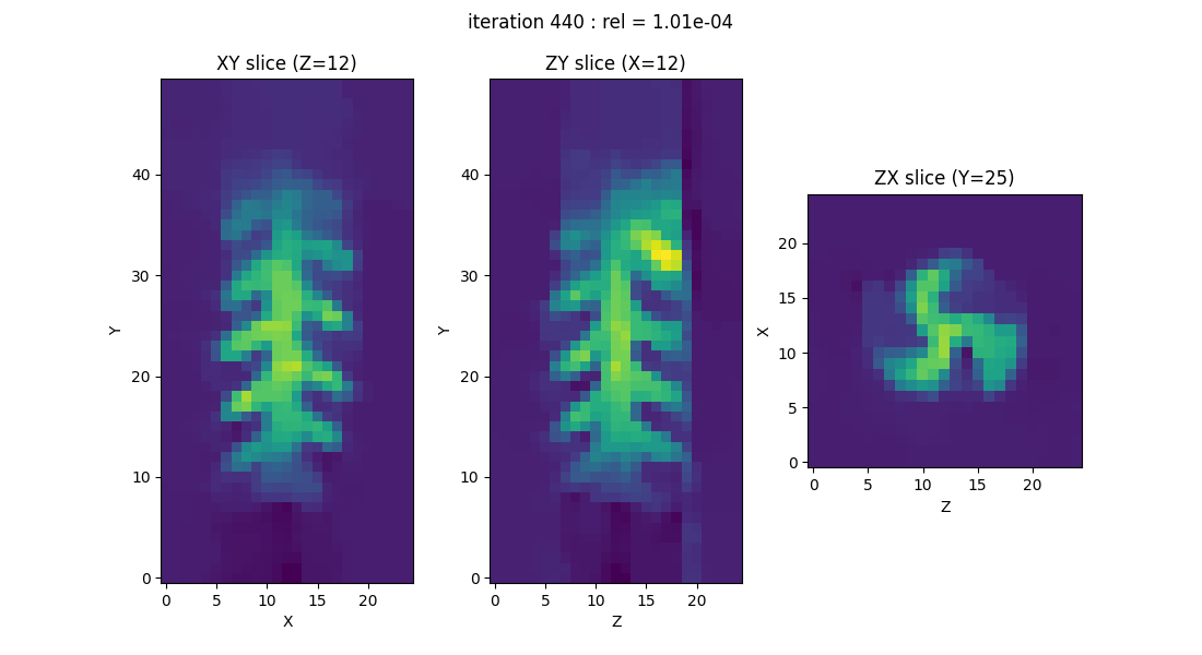
displayer = displayers.create_3d_displayer(nsrc=1, figsize=(11., 6.), display_labels=True)
out = processing.tv_monosrc(proj, B, fgrad, delta, h, lbda, out_shape, backend=backend,
                            init=None, tol=1e-4, nitermax=500, eval_energy=False,
                            verbose=False, video=True, Ndisplay=20, displayer=displayer)

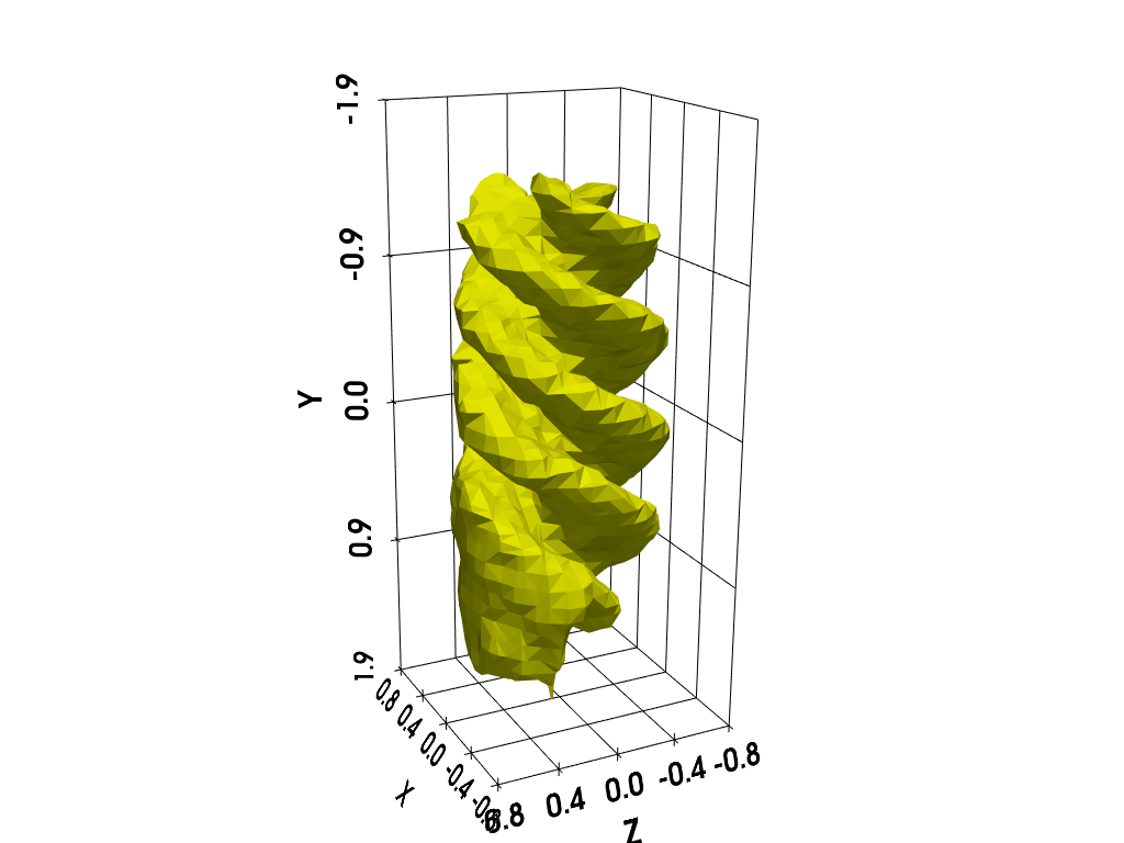
Basic Isosurface rendering (PyVista)

You can use the following code to “manually” compute and display an isosurface of the 3D image using PyVista.

# additional imports
import numpy as np
import pyvista as pv # tools for rendering 3D volumes
from pyepri.utils import otsu_threshold # used for automatic isovalue computation

# prepare isosurface display
xgrid = (-(out_shape[1]//2) + np.arange(out_shape[1])) * delta # X-axis (horizontal) sampling grid
ygrid = (-(out_shape[0]//2) + np.arange(out_shape[0])) * delta # Y-axis (vertical) sampling grid
zgrid = (-(out_shape[2]//2) + np.arange(out_shape[2])) * delta # Z-axis (depth) sampling grid
x, y, z = np.meshgrid(xgrid, ygrid, zgrid, indexing='xy')
grid = pv.StructuredGrid(x, y, z)

# compute isosurface
vol = np.moveaxis(backend.to_numpy(out), (0,1,2), (2,1,0))
grid["vol"] = vol.flatten()
isolevel = otsu_threshold(vol) # change the value here if needed (e.g., isolevel = .5 * vol.max())
contours = grid.contour(isolevel)

# display isosurface
cpos = [(-8.2, -3.1, 4.1), (0.0, 0.0, 0.0), (0.3, -0.95, -0.14)]
p = pv.Plotter()
p.camera_position = cpos
labels = dict(ztitle='Z', xtitle='X', ytitle='Y')
p.add_mesh(contours, show_scalar_bar=False, color='#f7fe00')
p.show_grid(**labels, bounds=[-0.8, 0.8, -1.9, 1.9, -0.8, 0.8])
p.show()

Static Scene

Interactive Scene

Interactive slices displayer (Matplotlib)

Use pyepri.displayers.imshow3d() to display the isosurface and slices of the 3D images using PyVista. Make sure the Matplotlib window has focus, then press the h key on your keyboard to display the list of interactive commands in your Python console.

Note: the slice selectors (sliders) won’t be active on this online documentation, but they should work when running the code on your system.

fig = displayers.imshow3d(backend.to_numpy(out), xgrid=xgrid, ygrid=ygrid, zgrid=zgrid, units='cm', figsize=(14.5, 8.8))

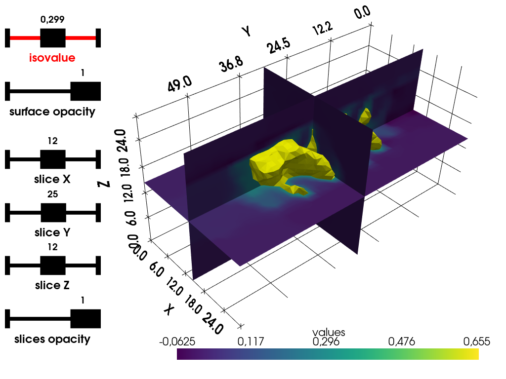
Interactive isosurface + slices displayer (PyVista)

Use pyepri.displayers.isosurf3d() to display isosurface and slices of the 3D images using PyVista, press key h on your keyboard to display the list of interactive commands into your Python console.

Notes:

• The slice images are rendered using bilinear interpolation, which results in overly smooth rendering near the edges of the objects.

• The widgets (here, sliders) will be disabled on the interactive view of this online documentation, but they should work when running the code on your system (either using Python console or Jupyter Notebook).

plotter = displayers.isosurf3d(backend.to_numpy(out))

Static Scene

Interactive Scene

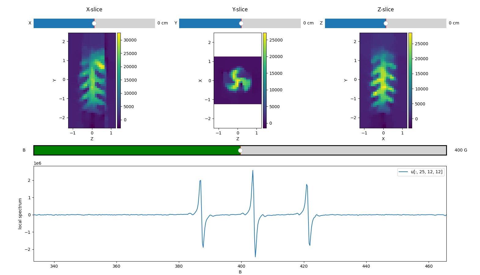
Interactive 4D spectral-spatial images viewer (matplotlib)

Below, we compute a 4D spectral spatial image by simply multiplying each voxel of the 3D image (concentration mapping) computed above by the reference spectrum.

im4d = h.reshape(-1, 1, 1, 1) * out.reshape((1, *out.shape)) # im4d[:, i, j, k] = spectrum
                                                             # at voxel location [i, j, k]

You can use pyepri.displayers.imshow4d() to display the contents of the 4D image. The spectrum corresponding to the voxel currently under the mouse cursor is shown in the lower panel. When you click on a voxel, its spectrum is preserved. Press h while the window is focused to display the full list of interactive commands.

Note: again, the slice selectors (sliders) won’t be active on this online documentation, but they should work when running the code on your system.

fig = displayers.imshow4d(backend.to_numpy(im4d), xgrid=xgrid, ygrid=ygrid, zgrid=zgrid,
                          Bgrid=backend.to_numpy(B), B_unit='G', spatial_unit='cm',
                          figsize=(15.7, 9))

Estimated memory usage: 543 MB